80 Essential Deep Learning Interview Questions (61-80)

This is Part 4 of a 4-part series covering 80 essential deep learning interview questions. Questions 61–80 cover applied and system-design questions: self-driving vehicles, medical imaging, production ML, and end-to-end system architecture.

Study tip: Applied questions test whether you can connect theory to real-world constraints — latency, data privacy, class imbalance, model monitoring. Always discuss tradeoffs, not just one “best” approach.

---

🚗 61. How would you approach building a deep learning model for self-driving cars?

Building a deep learning model for self-driving cars involves a multi-faceted approach. Let’s dive into the key components and practical strategies for each one.

Key Components

1. Perception and Classification: Uses sensors to perceive the driving environment.
2. Behavioral Planning: Decides on tasks such as lane keeping, overtaking, and turn signals.
3. Trajectory Planning: Plans the vehicle’s path based on the driving environment.
4. Low-Level Control: Executes commands such as steering and acceleration or braking.

Detailed Approach

1. Perception and Classification

• Camera: For lane detection, object detection, and sign recognition. You can use methods such as YOLO (You Only Look Once) or SSD (Single Shot Multibox Detector). YOLO is preferred in real-time settings.
• LiDAR: To create a 3D map of the surroundings, useful for obstacle detection and avoidance. Object detection would typically be done using point clouds.
• Radar: Used in adverse weather conditions.

2. Behavioral Planning

• DNN Integration: Use deep neural networks to process camera, LiDAR, and Radar data to make high-level decisions for behavioral planning, such as overtaking, following a lead vehicle, merging in traffic, etc.
• Path Planning Algorithms: Implement A* and other grid-based path planners for basic functions like obstacle avoidance and lane keeping.

3. Trajectory Planning

• Smooth Path Generation: Methods like the cubic spline or piecewise Bezier curves ensure gentle vehicle maneuvers.
• Object Prediction: Estimate future positions of moving objects to make trajectory plans that consider object movement.

4. Low-Level Control

• Vehicle Dynamics: Consider the vehicle’s dynamics, such as turning radii and maximum achievable accelerations, in the trajectory planning process.
• Follow-Up Control: Basic level controls, like PID controllers or model predictive controllers, ensure the vehicle maintains the desired trajectory.

Toolkits and Frameworks

• OpenCV: For image and video processing.
• TensorFlow / Keras: Ideal for building the deep learning stack.
• Carla or AirSim: Simulators that help in validating the model in virtual environments before deployment.

62. Propose a strategy for developing a deep learning system for medical image diagnosis.

When developing a Deep Learning system for Medical Image Diagnosis, it’s crucial to prioritize accuracy, interpretability, and ethics. Here’s a multi-stage approach that balances these priorities:

Data Collection

• Quantity: Aim for a diverse, large, and balanced dataset.
• Quality: Engage skilled annotators and utilize high-resolution images.
• Ethics: Collect data in a GDPR and HIPAA-compliant manner with patient consent.

Model Selection and Interpretability

• Model Choice: Consider using pre-trained models like DenseNet or Inception, tailored to medical imaging tasks. These architectures, like DenseNet, optimize for feature reuse and can benefit from transfer learning.
• Explainable AI: Adopt techniques such as Grad-CAM for better transparency in model predictions.

Fine-Tuning and Model Evaluation

• Transfer Learning: Start with a pre-trained model and update its weights using your dataset to save computational resources and time.
• Data Augmentation: Apply transformations like rotation, scaling, and flipping to enhance the dataset and augment the model’s robustness.
• Systematic Validation: Divert a portion of the data to be used for validation, and when approaching model evaluation, consider using k-fold or stratified cross-validation.

Post-training Analysis

• Error Analysis: Examine instances where the model was incorrect to identify misclassifications and build a roadmap for improvement.
• Model Calibration: Use methods like Platt Scaling or Isotonic Regression to make the confidence scores of the model align better with actual probabilities.

Domain and Social Considerations

• Expert Integration: If possible, deploy a system that incorporates human expertise in a dual-review mechanism.
• Fairness and Bias: Analyze your model for biases and inequalities and employ strategies to correct them; adjust the decision thresholds for the model.
• Transparency: Reaffirm the model’s credibility, making sure to clearly outline its capabilities and limitations. This transparency is vital in a medical setting.

63. Describe the steps you would take to create a recommendation system using deep learning.

Building a recommendation system with deep learning involves several key steps, from data preparation to model evaluation.

Key Components

1. Data Gathering: Collect user and item interaction data.
2. Preprocessing: Handle missing values and tokenize text.
3. Modeling: Construct a deep learning model.
4. Training: Use stochastic gradient descent to optimize the model’s loss function.
5. Evaluation: Run the model on test datasets and evaluate its performance.

Data Preparation

1. User-Item Matrix: In traditional recommendation systems, data often exists in a “user-item” matrix where each cell indicates a user’s interaction with an item (e.g., purchase, rating).
2. Interaction Representation: Convert interactions (e.g., ratings, clicks) into the form most suitable for the neural network. For textual data, this may involve tokenizing user or item descriptions.

The Model Architecture

1. Base Neural Network: X for user interactions with other items and vice versa. X is then concatenated with other user and item features before being input into a neural network.

2. Neural Collaborative Filtering (NCF): Combines the best of RNNs and MLPs for sequence learning and more direct relationships.

3. Autoencoders: Train the neural network to minimize input-output differences, and use the encoder to generate the latent space representations before applying the dot product to get rankings for a user.

Training

• Setup: Divide the data into training, validation, and test sets.
• Optimizer: Use algorithms like Adam or RMSProp for better convergence.
• Loss Function: Apply customized loss functions that consider the problem, such as ranking-aware losses for implicit feedback.

Evaluation

• Metrics:
  • Root Mean Square Error (RMSE) and Mean Absolute Error (MAE) for explicit feedback.
  • Area under the ROC curve (AUC) and F1 score for implicit feedback.
  • Top-K accuracy for recommended lists.
  • NDCG for ranked lists.
• Validation Set: Use it to tune hyperparameters.
• Test Set: Final assessment to see how the model performs on unseen data.

Potential Challenges

1. Cold Start Problem: How do you provide recommendations for new users or items with limited data?

2. Data Sparsity: What if you have limited data for some users or items?

3. Hyperparameter Tuning: There might be numerous neural network, training, and other hyperparameters to tune.

4. Data and Model Scaling: Deep learning models typically require more significant amounts of data to train effectively, and they also tend to be more computationally intensive.

Code Example: PyTorch - NCF Model

Here is the Python code:

import torch
import torch.nn as nn

class NCF(nn.Module):
    def __init__(self, num_users, num_items, embedding_dim, hidden_dim):
        super(NCF, self).__init__()
        self.user_embedding = nn.Embedding(num_users, embedding_dim)
        self.item_embedding = nn.Embedding(num_items, embedding_dim)
        self.mlp = nn.Sequential(
            nn.Linear(2 * embedding_dim, hidden_dim),
            nn.ReLU(),
            nn.Linear(hidden_dim, 1)
        )
        self.sim = nn.Sigmoid()

    def forward(self, user, item):
        user_embed = self.user_embedding(user)
        item_embed = self.item_embedding(item)
        mlp_input = torch.cat((user_embed, item_embed), 1)
        mlp_out = self.mlp(mlp_input)
        return self.sim(mlp_out)

In this model, we embed user and item IDs and then concatenate these embeddings as input to a multi-layer perceptron (MLP) before finally passing it through a sigmoid activation to obtain a predicted interaction.

64. How would you design a neural network to predict stock prices using time-series data?

Building a neural network (NN) to predict stock prices involves addressing several key challenges. I will use a Recurrent Neural Network, specifically an Long Short-Term Memory (LSTM), as its architecture is well-suited for time-series data.

Key Components of LSTM

• Input Layer: Accepts time steps as sequential input.
• Hidden State: Maintains contextual information from previous time steps.
• Memory Cell: Utilizes gating functions to regulate information over time.

Design Considerations for Stock Price Prediction

Data Preprocessing

1. Scaling: Normalize the data for values between 0 and 1 or using Z-score.
2. Sequencing: Group data in time windows or sequences to create XX and YY pairs for training.

Model Architecture

• Input Layer: Suitable size based on how many time steps you consider for prediction.
• Hidden Layers: Can consist of multiple LSTM or other types of layers, such as dense layers.
• Output Layer: Single node for regression, predicting the next time step.

Training & Evaluation

• Optimizer: Use Adam optimizer for efficient training.
• Loss Function: Common choices include Mean Squared Error (MSE) for regression tasks.
• Metrics: Use classic metrics like RMSE, and consider including extra evaluation, such as “gain” metrics, that are more pertinent in financial domains. Always differentiate between the training and testing phase.

Python Code Example: LSTM for Stock Prediction

Here is the Python code:

from tensorflow.keras.models import Sequential
from tensorflow.keras.layers import LSTM, Dense
from tensorflow.keras.optimizers import Adam

# Set necessary parameters
n_lag = 3  # Number of time steps to consider
n_features = 1  # Univariate series
n_units = 50  # Number of units in LSTM cell

# Instantiate the model
model = Sequential()
model.add(LSTM(n_units, input_shape=(n_lag, n_features)))
model.add(Dense(1))

# Compile the model
model.compile(optimizer='adam', loss='mean_squared_error')

65. Discuss a deep learning approach to real-time object detection in videos.

When it comes to real-time object detection in videos, several deep learning models excel at this task. These include Region-based Convolutional Neural Networks (R-CNN), Faster R-CNN, and You Only Look Once (YOLO).

YOLO: A One-Step Detector

YOLO, a pioneer in real-time object detection, operates as a single forward pass through the network. This strategy makes it extremely fast, especially compared to traditional two-stage detectors like R-CNN family.

Network Architecture

The network is essentially a fully-convolutional neural network (FCNN) connected to a grid of bounding box predictors. Specifically, YOLO partitions the input image into a grid, each cell predicting a fixed number of bounding boxes and corresponding class probabilities.

YOLO Algorithm

The core algorithm utilizes a joint loss function, considering both localization and classification. This approach simplifies training and enables direct end-to-end optimization.

YOLO was also among the first models to introduce the concept of Intersection over Union (IoU) threshold to handle overlapping bounding boxes.

YOLO Variants

The original YOLO model has since evolved through several versions, each refining its core algorithms and architecture. Variants include YOLOv2, YOLO9000, and YOLOv3, integrating features like multi-scale prediction and improved computational efficiency. The most recent model is YOLOv4.

66. Present a framework for voice command recognition using a deep neural network.

Deep Neural Networks (DNNs), especially Recurrent Neural Networks (RNNs), have notably advanced the field of voice command recognition.

Core Components

1. Audio Feature Extraction: Convert audio data into a representation suitable for DNNs.
2. DNN Architecture: Tailor the network for audio classification.
3. Training Pipeline: Utilize techniques such as mini-batch training.
4. Deployment: Implement a real-time voice command recognizer.

Featured Techniques

Spectrogram Generation

For Classification and Preprocessing, Mel Frequency Cepstral Coefficients (MFCCs) or Short-Time Fourier Transforms (STFTs) can be used to convert audio samples into spectrograms.

Network Architecture

Design a custom RNN, using Long Short-Term Memory (LSTM) or Gated Recurrent Unit (GRU) cells, to provide memory for time-series data.

Optimizers and Regularization

For Model Tuning, techniques like dropout, early stopping, learning rate scheduling, and adaptive optimizers can be employed.

Model Evaluation

For Model Evaluation, precision, recall, F1 score, and ROC-AUC provide comprehensive performance metrics.

Code Example: Spectrogram Generation

Here is the Python code:

import numpy as np
import librosa

# Load audio file
audio, sr = librosa.load('audio.wav', sr=None)

# Compute STFT
stft = np.abs(librosa.stft(audio))

# Convert to Mel frequency scale
mel_spec = librosa.feature.melspectrogram(S=stft**2)

# Log-amplitude scaling
log_mel_spec = librosa.power_to_db(mel_spec)

Next Steps

1. Data Collection: Gather a dataset of voice commands.
2. Preprocessing: Convert audio files into the desired spectrogram format.
3. Model Development: Build and train a custom RNN for voice command recognition.
4. Evaluation: Assess the model’s performance on a test set.
5. Deployment: Implement the model in an application or device.

Best Practices

• Data Augmentation: Modify the training data by adding noise or changing pitch, enhancing the model’s robustness.
• Hyperparameter Tuning: Fine-tune the model’s parameters to boost performance.
• Real-time Predictions: Deploy the model to generate predictions instantaneously in applications or on devices.

Ethical Considerations

• Privacy: Safeguard users’ data and gain consent before gathering audio samples.
• Transparency: Declare the rationale for audio collection and provide users with an opt-out choice.
• Fairness: Guarantee the model is impartial in recognizing diverse voices and accents.

Tools and Libraries

• LibROSA: A Python library for audio and music analysis.
• TensorFlow/Keras: For streamlined DNN development and training.

67. How would you use deep learning to improve natural language understanding in chatbots?

Deep Learning has revolutionized Natural Language Understanding (NLU) for chatbots, enabling more accurate text interpretation.

Key Components in a Chatbot

• Intent Recognition: Classifies user input to derive the intent behind their message.
• Named Entity Recognition (NER): Identifies specific entities within the input, such as dates, locations, or product names.
• Slot Filling: Extracts additional details surrounding the recognized intent.

Main Techniques

1. Embeddings: These dense vector representations map words or phrases to high-dimensional spaces, capturing semantic relationships.

2. Attention Mechanisms: Crucial for understanding context and selective focus during text processing.

3. Recurrent Neural Networks (RNNs): Suitable for managing sequential data, making them practical for chatbot training.

4. Transformers: Particularly effective in recognizing long-range dependencies and are a suitable choice for chatbot design.

5. Generative Models: These are utilized in chatbots that generate free-form text such as responses.

6. Transfer Learning: By leveraging pretrained models, chatbots can be more efficient and accurate even with limited training data.

Neural Techniques in NLU

• Slot Filling and Intent Recognition: Bidirectional LSTMs enhance sequence learning, while attention mechanisms ensure context consideration.

• Entity Recognition and Coreference Resolution: RNNs, LSTMs, or transformer variants improve entity understanding, especially in conversations.

• Disambiguation and Understanding Connotations: Contextual word embeddings, such as BERT, help chatbots determine the precise meaning of words.

• Emotion and Sentiment Analysis: Models like BERT and EmoBERT provide insights into the user’s sentiments and demeanor, enabling the chatbot to respond more empathetically.

Code Example: Using BERT for Intent Recognition

Here is the Python code:

# Import BERT model for intent recognition
from transformers import BertForTokenClassification

# Load pre-trained BERT for intent classification
model = BertForTokenClassification.from_pretrained('bert-base-uncased', num_labels=num_labels)

# tokenize user input
tokens = tokenizer.encode(user_input, return_tensors='pt')

# perform intent classification
outputs = model(tokens)
predicted_intents = [np.argmax(out, axis=1).tolist() for out in outputs]

In the code, num_labels is the number of intents being recognized, and tokenizer and model are from the transformers library.

68. Outline a plan for using CNNs to monitor and classify satellite imagery.

Using Convolutional Neural Networks (CNNs) for satellite image monitoring and classification can involve several key stages:

1. Data Acquisition

Consult NASA’s Worldview, Landsat or Sentinel-Hub to access up-to-date satellite imagery in a variety of bands like visible, near-infrared, or thermal.

2. Data Pre-Processing

• Resampling: Ensure all bands have the same resolution.
• Normalizing: Standardize pixel values across bands.
• Mosaicking: Composite multiple images to cover a larger area.

3. Image Labelling

For supervised learning, images need to be annotated, often at the pixel or object level. Datasets like xView or SpaceNet provide labelled satellite images for various tasks.

4. Architecture and Model Selection

Choose a CNN model proven in remote sensing applications for features like:

• Strong feature extraction.
• Invariance to rotation and scale, characteristic of satellite imagery.
• Ability to focus: Useful for pinpointing areas or objects, such as buildings or farmland.
• Adaptation to spectral variety: Vital when inputs span different bands.

5. Model Training

Divide the data into training, validation, and test sets and employ best practices for CNN training:

• Use learning rate schedules to fine-tune the model.
• Implement early stopping to prevent overfitting.
• Decipher the need for transfer learning, especially if labelled satellite data is limited.

6. Model Evaluation

Accuracy, precision, and recall are fundamental but can be insufficient for rich, multilayered tasks. Other metrics include Cohen’s Kappa, F1-score, and Area Under the ROC Curve.

Consider using techniques like cross-validation to ensure robust performance.

7. Deploy and Monitor

Deploy the model to systematically receive, process, and interpret incoming data.

Use callbacks during training to monitor the model’s performance over time. This step is particularly crucial for its intended application in continuous satellite monitoring.

69. Describe an approach to develop a deep learning model for sentiment analysis on social media.

Sentiment analysis, styled after traditional NLP methods, has transformed with advanced deep learning techniques. When developing a deep learning model for sentiment analysis on social media, it’s essential to build the model in conjunction with robust text preprocessing procedures.

Preprocessing

1. Tokenization: Split text into individual words or units.

2. Normalization: Standardize text e.g., converting ‘US’ to ‘United States’.

3. Noise Reduction: Remove irrelevant text parts e.g., URLs, special characters, and excess whitespace.

4. Stopword Removal: Eliminate commonly used, yet non-informative words such as ‘the’, ‘and’, and ‘of’.

5. Lemmatization: Reduce words to their base or root form e.g., ‘running’ becomes ‘run’.

Feature Representation

The two primary methods for this are Bag-of-Words (BoW) and Word Embeddings.

BoW

BoW uses a vocabulary set to represent the text. Each word is a feature, and its presence or absence is the value.

Example Code:

Here is the Python code:

from sklearn.feature_extraction.text import CountVectorizer

# Sample data
corpus = [
    'This is the first document.',
    'This document is the second document.',
    'And this is the third one.',
    'Is this the first document?',
]

# Setting up the BoW vectorizer
vectorizer = CountVectorizer()

# Applying the vectorizer on the corpus
X = vectorizer.fit_transform(corpus)

# Review vocabulary and features
print(vectorizer.get_feature_names_out())
print(X.toarray())

Word Embeddings

Word embeddings, like Word2Vec and GloVe, transform words into high-dimensional vectors. These vectors carry semantic meaning and capture relationships between words.

Example Code:

Here is the Python code:

import gensim.downloader as api

# Load the Word2Vec model (may require internet connection)
word2vec_model = api.load('word2vec-google-news-300')

# Get the word vector for 'king'
word_vector = word2vec_model['king']

Model Building

A common choice for social media sentiment analysis is the Convolutional Neural Network (CNN) due to its capacity to recognize patterns in sequences.

Convolutional Neural Network

A CNN for text often starts with an embedding layer and then incorporates convolutional and pooling layers. This configuration can extract local and global features from text.

Example Code:

Here is the Python code:

from keras.layers import Embedding, Conv1D, GlobalMaxPooling1D
from keras.models import Sequential

# Instantiate the model
cnn_model = Sequential()

# Add the embedding layer
cnn_model.add(Embedding(input_dim=vocab_size, output_dim=embedding_dim, input_length=maxlen))

# Add a 1D convolutional layer
cnn_model.add(Conv1D(filters=32, kernel_size=3, padding='same', activation='relu'))

# Add a global max pooling layer
cnn_model.add(GlobalMaxPooling1D())

# Add a feed-forward neural network
# ...

# Compile the model
cnn_model.compile(optimizer='adam', loss='binary_crossentropy', metrics=['accuracy'])

# Print model summary
cnn_model.summary()

70. How can deep learning be applied in predicting genome sequences?

Applying deep learning to predict genome sequences primarily involves sequence-to-sequence models and 2D convolutional neural networks tailored for spatial input.

Data Representation

• DNA sequences are traditionally encoded in nucleotide bases (A, T, G, C).
• For deep learning, k-mers maintain adjacency information and the potential for attention mechanisms.
• When the sequence has associated annotations (like gene starts or protein binding sites), an extended alphabet is employed.

Sequence Models

• Encode the DNA sequence as a series of overlapping k-mer tokens.
• Use specialized attention or quantile-based approaches to handle long DNA sequences efficiently.

Architecture for Sequence Classification

One-Dimensional Convolution (1D CNN)

1D CNNs are useful for extracting local patterns in the sequence.

• Input shape: k-mers (segments of the genome).
• Output shape: 1 or 0 (binary classification for regulatory regions).

Recurrent Neural Networks (RNNs)

RNNs, particularly Long Short-Term Memory (LSTM) networks, are well-suited for capturing long-range dependencies in sequential data.

• Input shape: variable-length sequence of k-mers.
• Output shape: variable-length sequence of annotations.

2D Architectures

Matured DNA sequence data types, such as the ones from DeepSEA, are presented as multi-channel images.

Convolutional Neural Networks (CNNs)

CNNs with 2D convolutions have found extensive application in image data but can also be adapted to certain types of sequence data. These networks handle inputs structured as matrices or three-dimensional tensors, which aligns with how DNA sequences are transformed.

Convolutional Neural Networks for DNA Sequences (CNN-DNA)

Here are the steps to build this model:

1. Convert DNA sequences to numerical form.
2. Pad or truncate sequences to a uniform length.
3. Split sequences into k-mers and encode them.

from sklearn.preprocessing import OneHotEncoder

k_mer_length = 4
dna_mapping = {'A': 0, 'T': 1, 'G': 2, 'C': 3}
# Create all possible k-mers
all_kmers = [''.join(item) for item in product(['A', 'T', 'G', 'C'], repeat=k_mer_length)]
# Initialize one-hot encoder
enc = OneHotEncoder(sparse=False,  dtype=int)
enc.fit(all_kmers)
# Function to one-hot encode a sequence
def encode_sequence(seq, k_mer_length, mapping, encoder):
    kmers = [seq[i:i+k_mer_length] for i in range(0, len(seq)-k_mer_length+1)]
    encoded = []
    for kmer in kmers:
        encoded.append(list(encoder.transform([list(kmer)]).flatten()))
    return np.array(encoded)

# Example usage
sequence = "ATGCTGAC"
encoded = encode_sequence(sequence, k_mer_length, dna_mapping, enc)

1. Split encoded k-mers into sequences of fixed length (forming 2D input).

This results in a 2D input tensor, where the rows correspond to k-mers and the columns represent the nucleotides within a k-mer, one-hot encoded.

For instance:

\[\begin{matrix} \text{ATGC} & \text{GCTA} & \dots & \\ 1 & 0 & 0 & 0 \\ 0 & 1 & 0 & 0 \\ 0 & 0 & 1 & 0 \\ 0 & 0 & 0 & 1 \end{matrix}\]

Building a 2D DNA CNN

Here is the Python code:

from keras.models import Sequential
from keras.layers import Conv2D, MaxPool2D, Flatten, Dense

# Define the model
model = Sequential()
model.add(Conv2D(filters=64, kernel_size=4, activation='relu'))
model.add(MaxPool2D(pool_size=(2,2)))
model.add(Flatten())
model.add(Dense(1, activation='sigmoid'))

# Compile the model
model.compile(optimizer='adam', loss='binary_crossentropy', metrics=['accuracy'])

# Train the model
model.fit(X_train, y_train, validation_data=(X_val, y_val), epochs=10, batch_size=32)

71. How do you evaluate the performance of a deep learning model?

Evaluating Deep Learning models involves measuring their ability to generalize. Common techniques include cross-validation, train-test splits, and rigorous performance metrics such as accuracy, precision, recall and F1-score.

Key Performance Metrics

Accuracy (ACC)

\[\text{ACC} = \frac{\text{TP} + \text{TN}}{\text{TP} + \text{TN} + \text{FP} + \text{FN}}\]

Precision

\[\text{Precision} = \frac{\text{TP}}{\text{TP} + \text{FP}}\]

Recall (Sensitivity)

\[\text{Recall} = \frac{\text{TP}}{\text{TP} + \text{FN}}\]

F1-Score

\[\text{F1-Score} = 2 \times \frac{\text{Precision} \times \text{Recall}}{\text{Precision} + \text{Recall}}\]

Specificity (True Negative Rate)

\[\text{Specificity} = \frac{\text{TN}}{\text{TN} + \text{FP}}\]

Receiver Operating Characteristic (ROC) & Area Under the Curve (AUC)

• ROC curve: A graph showing the true positive rate against the false positive rate.
• AUC: The area under the ROC curve. An AUC of 1.0 represents a perfect model, while an AUC of 0.5 indicates a random classifier.

Visualizing ROC Curves:

Here is the Python code:

import matplotlib.pyplot as plt
from sklearn.metrics import roc_curve, roc_auc_score

# Assuming y_test and y_pred are defined
fpr, tpr, _ = roc_curve(y_test, y_pred)
plt.plot(fpr, tpr, label="ROC Curve")
plt.plot([0, 1], [0, 1], linestyle='--', label='Random')
plt.xlabel('False Positive Rate')
plt.ylabel('True Positive Rate')
plt.title('ROC Curve')
plt.show()

Confusion Matrix

A confusion matrix tabulates True Positives (TP), True Negatives (TN), False Positives (FP), and False Negatives (FN). It is especially useful for binary classification tasks.

Visualizing Confusion Matrices

Python code:

import seaborn as sns
from sklearn.metrics import confusion_matrix

# Assuming y_test and y_pred are defined
conf_mat = confusion_matrix(y_test, y_pred)
sns.heatmap(conf_mat, annot=True, cmap='Blues', fmt='g')
plt.xlabel('Predicted')
plt.ylabel('Actual')
plt.show()

Metrics for Multi-Class Classification

• Cohen’s Kappa adjusts for the possibility of correct predictions by chance, especially useful when classes aren’t balanced.
• Mean Squared Error (MSE) represents the average squared difference between the predicted and true values. It’s particularly suitable for regression problems.

Cross-Validation

Cross-validation combines multiple train-test splits for a more comprehensive evaluation. It’s especially useful when the dataset is limited.

Variants of Cross-Validation

• K-Fold: The dataset is divided into K subsets, and the process is repeated K times, with each subset serving as the test set once and the others as the training sets.
• Stratified K-Fold: Ensures that each fold is representative of the class proportions in the dataset.
• Leave-One-Out: Each sample is used as a test set once.
• Time Series Split: For temporal data, ensures that the training and test sets are based on time.

Practical Considerations

• Model Complexity: Be mindful of overfitting; a high accuracy on the training set might not generalize well.
• Unbalanced Datasets: Metrics such as precision and recall are better choices when classes are skewed.

72. What techniques are used for visualizing and interpreting deep neural networks?

Deep neural networks can be complex and opaque, making it hard to understand why they make certain predictions. A range of techniques assist in the visual and interpretation of these models.

Techniques for Visualizing Deep Learning Models

Class Activation Maps (CAM)

Here is the Python code:

import numpy as np
import cv2
from keras.applications.resnet50 import preprocess_input
from keras.preprocessing import image
from keras.applications.resnet50 import ResNet50, decode_predictions

# Load the pre-trained ResNet50 model
model = ResNet50(weights='imagenet')
# Choose a specific layer for visualization, for ResNet50, usually the last convolutional layer is a good choice.
last_conv_layer = model.get_layer('activation_49')

# This is the input to the last convolutional layer
classifier_input = model.input

# Obtain the gradients of the last conv layer with respect to the prediction output
# This gives you how sensitive each output is to the convolutional layer features
grads = K.gradients(model.output[:, class_index], last_conv_layer.output)[0]

# Pool the gradients to determine the importance of each map in the convolutional layer
pooled_grads = K.mean(grads, axis=(0, 1, 2))

# Combine the conv layer output and the gradients
iterate = K.function([model.input], [pooled_grads, last_conv_layer.output[0]])
pooled_grad_value, conv_layer_output_value = iterate([np.array([input_image])])

# Give importance to the map
for i in range(1):
    conv_layer_output_value[:, :, i] *= pooled_grad_value[i]

CAM focuses on the relevant area in an image that influences the model’s prediction. By overlaying this information on the image, it’s possible to understand which features in the image are critical.

Saliency Maps

• To generate a saliency map:

from keras import backend as K

inputs = [model.input]
output = model.output

# Calculate the gradients of output with respect to input
grads = K.gradients(output, inputs)[0]

# Compute the mean gradient
gradient_function = K.function(inputs, [grads])
grads_val = gradient_function([np.array([input_image])])[0]

# Plot the map to highlight the salient features
saliency = np.max(np.abs(grads_val), axis=-1)

Visualizing Embeddings

In the deep learning domain, “embeddings” generally refers to a space where input data has been learned and projected. Here are the code snippets:

• t-SNE: T-distributed stochastic neighbor embedding is a popular technique:

from sklearn.manifold import TSNE

# Assuming trained_data_features is the extracted feature vector from a trained DNN
X_embedded = TSNE(n_components=2).fit_transform(trained_data_features)

• PCA: Principal Component Analysis can be applied as well:

from sklearn.decomposition import PCA

pca = PCA(n_components=2)
principalComponents = pca.fit_transform(trained_data_features)

Understanding Feature Importance

For Deep Neural Networks, each input (pixel in an image, word in a sentence, etc.) gets assigned a weight that indicates its importance. For example, in computer vision, higher weights indicate image regions relevant to a certain class. Such weight visualization is commonly done for CNNs.

Here is the Python code:

import matplotlib.pyplot as plt

# Normalize the weights
weights = (weights - np.mean(weights)) / np.std(weights)

# Plot the normalized weights in context of the input image
plt.matshow(weights, cmap='viridis')
plt.show()

Misclassified Examples

Sometimes, misclassified examples of a model can provide insight into why the model got it wrong. Visualizing these examples can be a method of detecting systematic issues.

Here is the Python code:

import numpy as np
import matplotlib.pyplot as plt

incorrect_indices = np.where(predicted_classes != true_classes)[0]
# Displaying a few misclassified examples
for i in range(6):
    plt.subplot(2, 3, i + 1)
    # Reshape the image data if needed
    plt.imshow(images[incorrect_indices[i]])
    plt.title("Predicted:{}\nTrue:{}".format(predicted_classes[incorrect_indices[i]], true_classes[incorrect_indices[i]]))
plt.show()

73. Discuss the methods for handling a model that has a high variance.

When a model has high variance, it means that it’s overly complex or has been overfit to the training data. Such a model tends to perform well on the training data but poorly on unseen data.

Techniques for Reducing Variance

1. Regularization: Techniques like L1 (LASSO) or L2 (Ridge) regularization add penalty terms to the loss function, discouraging overly complex models. The strength of the penalty is controlled by a hyperparameter.

2. Ensemble Methods: Using a group of diverse models can improve overall performance, balancing each model’s strengths and weaknesses.

   • Bagging: Random Forest integrates predictions from multiple decision trees trained on subsamples of the data.
   • Boosting: Algorithms like AdaBoost train models iteratively, with more emphasis on previously misclassified instances.

3. Cross-Validation: Instead of using a single fixed dataset for validation, techniques such as K-fold cross-validation or leave-one-out validation provide more reliable performance estimates by utilizing the entire dataset for both training and validation.

4. Hyperparameter Tuning: Adjusting the hyperparameters of the learning algorithm (e.g., learning rate, tree depth, degree of polynomial features) can help control model complexity and reduce variance.

5. Early Stopping: This technique involves monitoring model performance on a validation set during training. When performance starts to degrade, training is halted to prevent overfitting.

6. Feature Selection: Reducing the number of features can help simplify the model and reduce overfitting.

7. Feature Engineering: Crafting meaningful features that convey more information to the model can enhance generalization.

8. Model Selection: Sometimes, a simpler model is preferred, especially in cases involving limited data or when the computational cost of a complex model is prohibitive.

9. Data Augmentation: For image or text data, techniques like horizontal/vertical flips, rotations, slight zooms, or paraphrasing can increase the diversity of data seen by the model during training.

10. Dropout: Commonly used in neural networks, dropout involves randomly “dropping out” (setting to zero) neurons in the model during training to reduce interdependence and overfitting.

74. How can confusion matrices help in the evaluation of classification models?

In the context of evaluating classification models, the primary tasks are to understand the various types of model predictions and to compare them with the ground truth. A Confusion Matrix serves as a comprehensive tool for these evaluations.

Core Components

• True Positives (TP): The model correctly predicted the positive class.
• True Negatives (TN): The model correctly predicted the negative class.
• False Positives (FP): The model incorrectly predicted the positive class when it was actually negative.
• False Negatives (FN): The model incorrectly predicted the negative class when it was actually positive.

Calculation Metrics

From these core components, we can calculate key evaluation metrics including precision, recall, F1-score, and accuracy.

Precision

Precision is a measure of the accuracy provided that a specific class has been predicted.

\[\text{Precision} = \frac{\text{True Positives}}{\text{True Positives} + \text{False Positives}}\]

Recall (Sensitivity)

Recall is the true positive rate and measures the ratio of actual positives that are correctly predicted.

\[\text{Recall} = \frac{\text{True Positives}}{\text{True Positives} + \text{False Negatives}}\]

F1-Score

The F1-score is the harmonic mean of precision and recall.

\[\text{F1-score} = 2 \times \left( \frac{\text{Precision} \times \text{Recall}}{\text{Precision} + \text{Recall}} \right)\]

Accuracy

Accuracy is a measure of the overall correctness of a model’s predictions.

\[\text{Accuracy} = \frac{\text{True Positives} + \text{True Negatives}}{\text{True Positives} + \text{True Negatives} + \text{False Positives} + \text{False Negatives}}\]

75. Explain the significance of ROC curves and AUC in model performance.

The Receiver Operating Characteristic (ROC) Curve and its Area Under the Curve (AUC) are key components of models’ predictive performance analysis.

ROC Curve: Understanding TPR and FPR

The ROC curve provides a visual representation of a classifier’s performance across different classification thresholds. It plots the True Positive Rate (TPR) =TPTP+FN=\frac{{TP}}{{TP+FN}}, also known as recall, against the False Positive Rate (FPR) =FPFP+TN=\frac{{FP}}{{FP+TN}}, often associated with the Type 1 error.

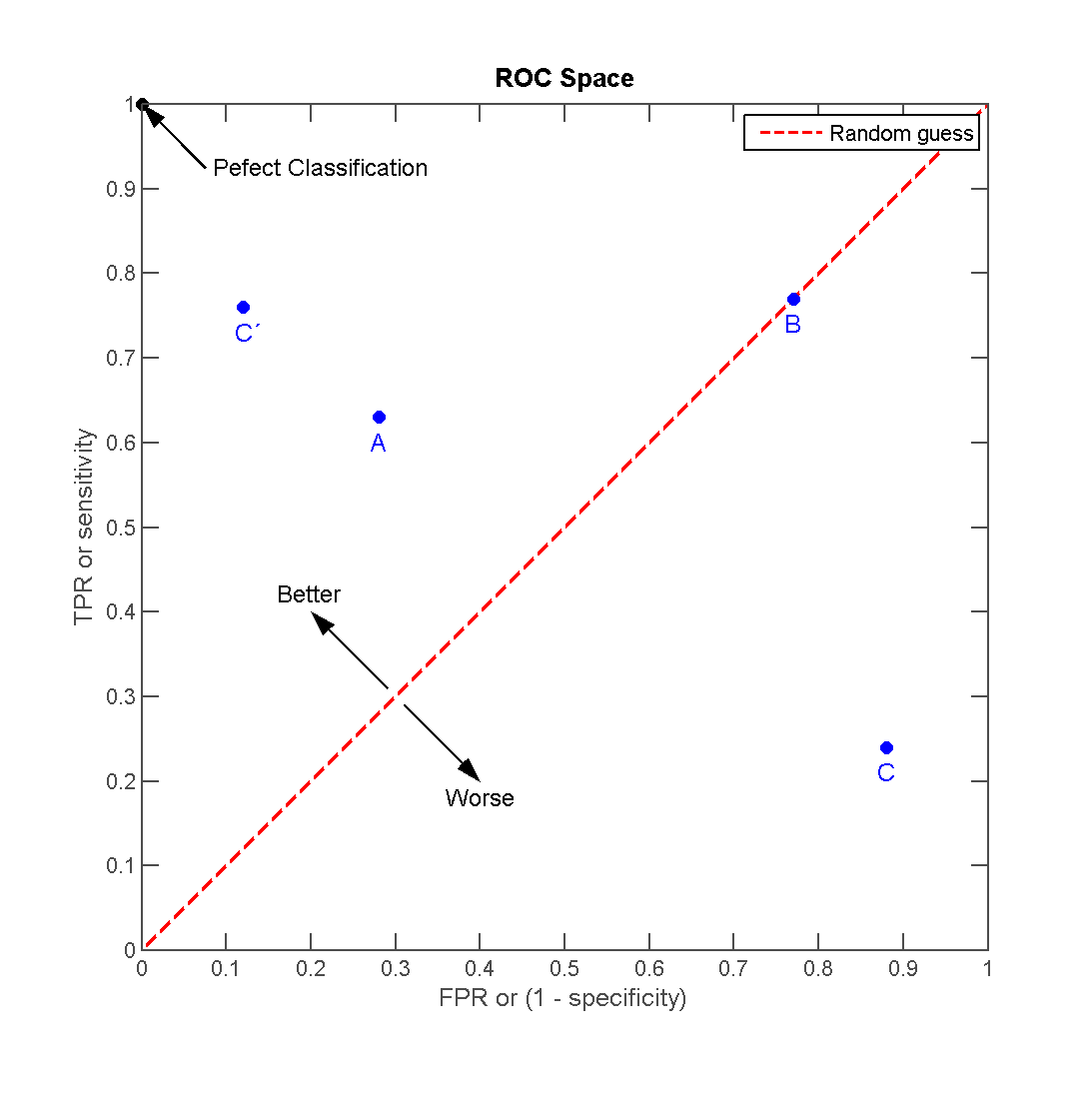
The ideal point on the ROC curve is (0,1) (0,1) , representing 100% TPR and 0% FPR, indicating perfect classification. Conversely, the point (1,0) (1,0) symbolizes total misclassification, 0% TPR, and 100% FPR.

The diagonal line from (0,0) (0,0) to (1,1) (1,1) signifies a random classifier.

AUC: Robustness and Predictive Power

The Area Under the ROC Curve (AUC) quantifies the capacity of a classifier to rank the samples across the predicted outcome probabilities. It is indeed the probability that a classifier would place a random positive sample ahead of a random negative sample.

The AUC ranges from 0 to 1. Higher AUC values suggest superior model classification.

• An AUC of 0.5 denotes a random and ineffective model.
• An AUC of 1.0 signifies a model that achieves perfect separation between the positive and negative classes.

Advantages

The ROC curve and AUC offer several advantages, such as:

• Threshold Agnosticism: The AUC computes a model’s accuracy across all feasible thresholds.
• Robustness Against Class Imbalance: AUC provides a reliable performance metric despite unequal class distribution.
• Model Comparisons: AUC allows for direct model comparisons, even in multi-class and probability thresholds settings.

76. What are the methods for model introspection and understanding feature importance in deep learning?

Understanding feature importance in traditional machine learning, especially for interpretable decision-making, has been one of the fundamental pillars of model evaluation and business analytics.

However, with deep learning, this process is more nuanced because of complex feature transformations occurring in hidden layers.

Techniques of Model Introspection and Feature Importance in Deep Learning

1. Activations Analysis: This method involves visualizing activations and exploring which neurons are most active for specific inputs. These visualizations can be insightful but are computationally expensive.

2. Saliency Maps: Popularized by techniques like CAM (Class Activation Maps), this method highlights regions of the input image that a network focuses on to make a particular decision.

3. Layer-Wise Relevance Propagation (LRP): LRP backward-propagates relevance scores from the output layer to the input layer, quantifying each pixel’s contribution.

4. Grad-CAM: This technique computes the gradient of the class score with respect to feature maps of a convolutional layer to generate a visual heatmap indicating regions of interest in the input.

Cons of Deep Learning

While each of these methodologies provides various degrees of insight, they often fall short of the interpretability and natural human-understanding levels seen in traditional models.

Deep learning models exhibit remarkable performance, especially in perceptual tasks like speech recognition and image classification. However, they somewhat lack the level of “explainability” that’s crucial in high-stakes or sensitive applications.

For instance, when a deep learning model designed to aid in medical diagnostics provides a positive diagnosis for an individual, it’s critical for healthcare professionals to understand why the model arrived at that decision.

A lack of transparency into the underlying decision-making process can erode trust, hinder regulatory compliance, and prevent deployment of such applications.

Model Complexity vs. Interpretability

The comprehensiveness of a model and its underlying mechanisms does not necessarily elucidate the mechanisms. Additionally, simpler or more interpretable models could potentially be enriched to include more features and remain intelligible.

Hybrid Approaches

Addressing the need for both high performance and interpretability, researchers have proposed hybrid models that combine the advantages of deep learning, such as feature learning, with the more transparent decision processes of traditional methods. These hybrid models aim to strike a balance between intelligence and interpretability.

77. How do you perform error analysis on the predictions of a deep learning model?

Error analysis is essential for understanding the performance of your deep learning model and identifying potential areas for improvement. Several techniques and tools can aid in this evaluation process.

Techniques for Error Analysis

Confusion Matrix

The confusion matrix provides a detailed breakdown of the model’s predictions, making it easier to detect false positives and false negatives. From this, you can assess metrics such as precision, recall, and the F1 score.

Visualizations

Data visualizations, such as precision-recall curves or ROC curves, are helpful for assessing model performance, especially for binary classification problems.

Individual Case Review

For more nuanced insights, you can explore individual instances where the model made mistakes and identify any patterns or commonalities.

Automated Reporting

Several tools automatically generate comprehensive error reports, which summarize the model’s performance and highlight potential issues.

Monte Carlo Dropout

This Bayesian approach uses dropout at inference time to sample multiple predictions for a single input and, consequently, estimate uncertainty in the model’s predictions.

Human-in-the-Loop

Even as AI systems continue to evolve, they are not yet foolproof. Human-in-the-loop systems can help validate and, if necessary, correct the AI’s predictions.

Code Example: Confusion Matrix

Here is the Python code:

from sklearn.metrics import confusion_matrix
import seaborn as sns
import matplotlib.pyplot as plt

# Assuming y_true and y_pred are your true and predicted labels
cm = confusion_matrix(y_true, y_pred)

# Visualize the confusion matrix with a heatmap
sns.heatmap(cm, annot=True, fmt="d")
plt.xlabel("Predicted")
plt.ylabel("True")
plt.show()

Notes on Deep Learning-Specific Challenges

• Data Quality: Convolutional Neural Networks (CNNs) can be biased if trained on images of differing quality.
• Transfer Learning Dynamics: When utilizing pre-trained models, it’s essential to gauge how well the learned representations apply to your specific task.
• Recurrent Neural Networks (RNNs) and Time Series: For sequence data, RNNs could struggle with long-range dependencies.
• Vanishing and Exploding Gradients: These are particular challenges when training deep networks with many layers. Techniques such as careful parameter initialization and advanced optimization methods can be employed to mitigate this issue.

78. Discuss the use of Precision-Recall curves and their importance.

Precision-Recall (PR) curves are among the most reliable evaluation tools, especially in imbalanced datasets. They showcase how model performance varies across different classification thresholds, offering a more nuanced view than the single-point metric of the F1-score.

Constructing the PR Curve

1. Threshold Selection: Vary the decision threshold of the classifier and for each threshold, calculate precision and recall.

2. Coordinate Plotting: Use precision as the y-axis and recall as the x-axis to plot the points (recall, precision) in the PR space.

3. Area Under the Curve (AUC): The PR curve’s AUC is a global measure of classifier performance.

PR Curve vs ROC Curve

While the Receiver Operating Characteristic (ROC) curve is adept at evaluating models across different operating points, the PR curve is better suited for imbalanced datasets as it ensures that both positive as well as negative classes are taken into account.

Imperfect Models

It’s also worth noting that the AUC of a PR curve can help assess model quality. For instance, if a classifier has an AUC near 0.50.5 on the PR curve, it mostly randomizes between Precision and Recall.

Code Example: Constructing a PR Curve

Here is the Python code:

from sklearn.metrics import precision_recall_curve
import matplotlib.pyplot as plt

# Assuming y_true and y_score are available
precision, recall, thresholds = precision_recall_curve(y_true, y_score)

plt.plot(recall, precision, marker='.')
plt.xlabel('Recall')
plt.ylabel('Precision')
plt.title('Precision-Recall Curve')
plt.show()

79. What is model explainability, and why is it important?

Model explainability refers to the ability to comprehend and interpret a machine learning model’s predictions. It is a crucial component in building reliable and ethical AI systems, especially when transparency and human intervention are required for decisions.

Importance of Model Explainability

• Ethics and Responsibility: In sensitive domains such as healthcare, finance, and justice, it’s critical to establish accountability and compliance with regulations. Interpretability aids in ensuring decisions are fair, transparent, and free from biases.

• Transparency and Trust: When human lives or privacy are at stake, stakeholders need to trust AI-driven systems. Explaining model outputs helps to establish trust by providing clear rationale behind decisions.

• Insight and Understanding: Interpreting a model can lead to new insights, potentially inspiring domain experts to investigate phenomena previously unrecognized or misunderstood.

• Detection and Remediation of Biases: Numerous models, if not carefully developed or handled, can inadvertently perpetuate, magnify, or legitimize existing biases. Model explainability assists in recognizing and rectifying such issues.

80. How do you deal with the interpretability-vs-performance trade-off in deep learning?

Deep learning methods are characterized by their high performance on complex tasks. However, this comes at the expense of interpretability, which refers to the model’s ability to explain its decisions in a human-understandable way.

Techniques for Improved Interpretability

• Simpler Architectures: Using standard, shallower networks can make models potentially more interpretable, although it’s often at the cost of performance.

• Ensembling: By combining predictions from multiple models, you can have improved certainty and also better interpretability, especially if the individual models are more straightforward.

• Feature Engineering and Reduction: Selecting or deriving the most relevant features for the task can help improve model interpretability.

• Hybrid Approaches: Use deep learning for feature extraction and traditional machine learning for the final decision-making.

• Optimized Hyperparameters: Optimized models with straightforward hyperparameters can be more interpretable.

• L1 Regularization: The nature of L1 regularization often results in sparser models, aiding in feature selection and interpretability.

• Dropout: While commonly used to fight overfitting, its stochastic nature can provide insight into the importance of various features, though this effect is less pronounced in larger networks.

• Global Explanation Methods: Techniques like LIME and SHAP can be used to understand individual predictions for complex models.

• Visualizations: Techniques like saliency maps, which indicate which parts of the input were most crucial for a particular prediction, can provide insight into the model’s workings.

Constraints in Different Industries

• Healthcare: Regulatory and ethical concerns often dictate the requirement for models to be interpretable.

• Finance: Interpretable models are necessary for regulatory compliance.

• Image and Speech Recognition: Tasks relying heavily on deep learning often focus more on performance than interpretability due to less regulation and the added challenge of interpreting complex data like images and sound.

Ethical Considerations

The lack of interpretability in deep learning can lead to opacity in decisions, raising ethical concerns in high-stakes scenarios such as medical diagnostics or criminal justice. These concerns have contributed to the recent push for more interpretable AI, leading to advancements in explanation techniques. Even so, sensitivity to the trade-off between interpretability and performance will continue to be a vital aspect of model development.

---

Part 4 of 4 — completing the 80 Essential Deep Learning Interview Questions series. Review all four parts for comprehensive interview preparation.