80 Essential Deep Learning Interview Questions (41-60)

This is Part 3 of a 4-part series covering 80 essential deep learning interview questions. Questions 41–60 cover adversarial robustness, attention mechanisms, transfer learning, and interpretability.

Study tip: Adversarial examples are a hot interview topic at safety-focused companies (Anthropic, DeepMind). Be able to explain FGSM mathematically and discuss at least two defense strategies.

---

⚔️ 41. What are adversarial examples in deep learning, and why do they pose a threat?

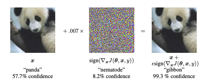
Adversarial examples are maliciously crafted inputs, often visually indistinguishable from their benign counterparts, that lead to misclassification when fed into machine learning models.

How Are They Created?

Adversarial examples are crafted using algorithms designed to exploit the weaknesses of deep learning models. Two common methods are:

1. Fast Gradient Sign Method (FGSM): Perturbing the input image in the direction that increases its loss the most. This is done by taking the sign of the gradient of the loss with respect to the input image and updating the image in that direction.

2. Projected Gradient Descent (PGD): Iteratively making small changes to the input image so that it remains misclassified.

Why Do They Pose a Threat?

Imperceptibility to Humans

Adversarial examples are crafted to be indistinguishable from benign inputs to the human eye, creating an especially insidious threat.

Repercussions in Real-world Deployments

The implications of adversarial attacks in various real-world applications like self-driving cars and security systems are severe. For instance, an adversarially perturbed stop sign might be misclassified by an autonomous vehicle.

Model Opacity

The existence of adversarial examples points to a lack of robustness in deep learning models. This very weakness might hinder the ability to fully comprehend and interpret such models.

Key Research and Defenses

Developing adversarial defenses is an active area of research. Examples include defensive distillation, adversarial training, and feature squeezing.

Despite the challenges, ongoing research seeks to understand the underlying principles better, thus advancing both the robustness and interpretability of deep learning models.

42. Discuss the concept of style transfer in deep learning.

Style transfer involves imbuing the artistic style of one image, known as the style image, onto another, termed the content image, creating a new image referred to as the stylized image.

The concept become popular following the work “A Neural Algorithm of Artistic Style” by Gatys, Ecker, and Bethge in 2015.

Key Components

• Style Representation: The preferred artistic style is typically quantified using a feature representation from a convolutional neural network (CNN).
• Content Representation: The visual content of the content image is also quantified using a network’s feature representation, often in a different layer than the one used for style.
• Loss Functions: Style transfer generally involves three distinct loss functions:
  • Style loss, which quantifies how well the stylized output matches the input style.
  • Content loss, which ensures that the content of the stylized image is similar to the content of the content image.
  • Total variation loss, which helps to reduce noise in the generated image.

Selecting the Style

There are different CNN layers that capture style features and useful for style representation:

• Gram Matrix: A statistical measure of feature correlations and is derived from intermediate CNN layers. It is calculated as an inner product of feature maps’ reshaped matrices.
• Correlation Between Entries: Encoded in feature maps computed by a CNN.

Mechanism

Traditional style transfer methods often utilize an optimization scheme to minimize the overall loss. However, a plethora of real-time style transfer techniques use modified network architectures that incorporate the style and content loss functions.

Visualize the Stylized Image

Here is the Python code:

import matplotlib.pyplot as plt

def plot_images(content_img, style_img, stylized_img):
    fig, ax = plt.subplots(1, 3, figsize=(10, 5))
    fig.suptitle('Style Transfer')

    ax[0].imshow(content_img)
    ax[0].set_title('Content Image')
    ax[0].axis('off')

    ax[1].imshow(style_img)
    ax[1].set_title('Style Image')
    ax[1].axis('off')

    ax[2].imshow(stylized_img)
    ax[2].set_title('Stylized Image')
    ax[2].axis('off')

    plt.show()

# Assuming content_img, style_img, and stylized_img are loaded images
plot_images(content_img, style_img, stylized_img)

43. What are the current challenges in training deep reinforcement learning models?

Training Deep Reinforcement Learning (DRL) models presents unique challenges due to the complexity of deep neural networks and the inherent difficulties in optimizing RL algorithms.

Challenges in Training DRL Models

• Sample Efficiency: DRL models typically require significantly more data samples to train effectively compared to supervised learning models. This is due to the temporal nature of the data and the potential for high variance, which can slow down the learning process.
• Stability and Exploration: Balancing exploration (trying out new actions to learn) with exploitation (choosing known good actions to earn rewards) is an ongoing challenge in DRL. Agents may get stuck in suboptimal policies or exhibit erratic behaviors due to a lack of robustness in exploration-exploitation strategies.
• Catastrophic Forgetting: Deep networks are susceptible to losing previously learned knowledge when exposed to new data. This can be problematic in the context of RL, especially in environments where the agent’s actions have long-term consequences or there’s a mix of long- and short-term tasks.
• Partial Observability: Many real-world tasks and environments provide only partial or noisy feedback. Agents must be capable of making decisions based on incomplete information, which demands advanced memory and information fusion techniques.
• Overfitting: Although not new to machine learning, overfitting is a critical challenge in DRL. Overfitting occurs when an agent has memorized specific sequences of actions and learned behaviors that are not generalizable.
• Credit Assignment: In environments with sparse or delayed rewards, determining which set of actions led to a positive outcome becomes more challenging. Proper credit assignment is crucial for the agent to learn an optimal policy.
• Reward Design: The design of the reward function heavily influences the learning process. A poorly designed reward function can lead to suboptimal or even unwanted behavior from the agent. Crafting well-designed reward functions often requires domain expertise.

Techniques to Address DRL Challenges

• Experience Replay: Buffers past transitions in a replay buffer, helping to mitigate issues such as catastrophic forgetting and enhance sample efficiency by enabling multiple learning opportunities from a single experience.
• Dueling Networks: Separates the Q-network into two streams to help distinguish between valuable and non-valuable actions, potentially improving sample efficiency and agent stability.
• Distributional RL: Tools such as Categorical-DQN help the agent better understand the distribution of expected returns for each action, potentially improving stability and sample efficiency.
• Continuous Control: While designed for continuous action spaces, these algorithms also work well for discrete spaces, potentially improving sample efficiency and stability.
• Actor-Critic Models: These hybrid models offer the best of both worlds, providing a combination of value-based and policy-based learning, potentially improving both stability and sample efficiency.
• Intrinsic Motivation: Incorporates means for the agent to be intrinsically motivated to explore, usually through auxiliary reward signals. This can help improve exploration strategies.

Future Directions

The field is rapidly evolving in the quest to make DRL more efficient and effective. Exciting research in Adversarial Training, Intrinsic Motivation, Bootstrapping, and more areas is actively tackling these challenges. The maturation of these methods, coupled with advancements in hardware, is poised to make DRL more widely applicable in the near future.

44. Explain the concept of few-shot learning and its significance in deep learning.

Few-shot learning in the context of deep learning refers to the ability of a model to make accurate predictions when provided with very limited training data. Traditional deep learning algorithms typically require substantial amounts of labeled data for effective training.

Few-shot learning plays a pivotal role in overcoming data scarcity and computationally intensive training in numerous real-world use cases.

Primer on Transfer Learning

Transfer learning serves as a foundation for Few-shot learning by leveraging existing knowledge from a source task to improve learning in a related target task. This obviates the need for extensive task-specific labeled datasets, which are often hard to obtain.

Popular methods such as one-shot learning and zero-shot learning expand on transfer learning, though they differ in their conduit and the amount of required training data.

One-Shot Learning

In one-shot learning, models are trained to make inferences after being presented with just one example per class, which is why it’s often visualized as learning tasks with just a solitary support example. While this approach is promising, achieving high accuracies from one example per class is a challenging feat, especially in complex domains.

Zero-Shot Learning

Zero-shot learning endeavors to make predictions for instances unseen during training. Instead of requiring the presence of an instance during the training phase, zero-shot models have knowledge about unseen or new classes. Techniques such as attribute-based classification or using textual descriptions for classes can enable zero-shot learning.

Generalized Few-Shot Learning

This technique, popularized by matching networks, equips models to generalize across tasks, therefore supporting more diverse predictions. Here, the model learns from more examples during testing by adjusting its hypothesis.

Practical Applications

Few-shot learning has been instrumental in a wide array of fields, from data science to computer vision, and natural language processing, offering innovative solutions in academia and industry.

• Medical Imaging: Efficient tumor detection from minimal scans.
• Data Augmentation: Generating synthetic data for training.
• Cross-Lingual Tasks: Making accurate translations with minimal language pairs.
• Content Recommendation: Precise suggestions with sparse user feedback.
• Voice Computing: Personalized and adaptable voice assistants.

Areas for Improvement

While remarkable, models for Few-shot learning can still be inconsistent and underperform in certain scenarios. There is ongoing research to address these limitations, often through enhanced meta-learning techniques that enable models to learn from fewer examples more effectively.

45. What are zero-shot learning and one-shot learning?

Zero-shot learning and one-shot learning offer solutions for tasks where labeled data may be scarce.

Zero-Shot Learning

In zero-shot learning, a model makes predictions without needing any examples from certain classes. Instead, it leverages intermediate information or extra data sources.

Example: Bird Classification

If a neural network is trained to recognize birds within a specific dataset but never before encountered an ostrich, it can still predict an image as that species by associating the keyword “ostrich” with additional attributes such as “large,” “flightless,” or “Africa.”

Methodologies

• Attribute-based recognition: Birds might be characterized by features like “beak shape,” “color,” or “habitat,” which allow a model to identify them based on these traits.

• Textual descriptions or natural language attributes: Instead of images, models can use textual attributes to make inferences.

• Relationship embeddings: This approach encodes relationships between images and their attributes, connecting the characteristics of images with their labels.

One-Shot Learning

In one-shot learning, models can learn to recognize classes with minimal examples, sometimes just one.

Example: Face Verification

Given a novel image, a model trained using one-shot learning can compare this image to a single reference image of the individual and ascertain whether they are the same person.

Methodologies

• Siamese Networks: This setup employs two identical neural networks, sharing the same weights and architecture. They accept distinct images for comparison and are trained to minimize a similarity metric.

• Metric Learning: Instead of directly classifying inputs, these models compute a similarity metric between pairs and optimize parameters to improve performance for known instances.

Hybrid Approaches

• Meta-learning: Also referred to as “learning to learn,” it trains models on multiple tasks rather than just one, allowing them to apply this knowledge to new, unseen tasks.

• Transfer Learning and Pre-training: These models are initially trained on a comprehensive dataset and then fine-tuned on a smaller one, leading to improved zero-shot and one-shot performance. For example, GPT-3, a pre-trained language model, demonstrates exceptional zero-shot learning abilities.

46. Discuss the role of deep learning in Natural Language Processing (NLP).

Deep Learning has transformed the field of Natural Language Processing (NLP), surpassing previous methods with its ability to learn abstract and hierarchical representations from textual data.

Key Components of Deep Learning in NLP

• Embeddings: Methods like Word2Vec and GloVe convert words into high-dimensional vectors, capturing semantic and syntactic relationships.

• Sequences: Dedicate structures such as Recurrent Neural Networks (RNNs) and Long Short-Term Memory (LSTM) networks process input sequences and remember context over time.

• Attention Mechanisms: Introduce adaptability by learning which parts of a text are most relevant or provide context to a specific task.

• Transformers: Contextualize words based on the entire sentence using self-attention. Their use led to significant advancements in many NLP tasks.

NLP Applications Enhanced by Deep Learning

• Machine Translation: Deep Learning has boosted translation quality significantly, especially with the introduction of sequence-to-sequence models.

• Sentiment Analysis: By capturing subtle nuances in text data, deep learning models improved the accuracy of sentiment classification tasks.

• Named Entity Recognition: State-of-the-art models now use advanced deep learning architectures to effectively identify entities within text.

• Text Generation: From language models to generative models like GPT-3, deep learning has enabled machines to produce human-like text.

• Question Answering: Deep learning models can decode questions, find relevant information within a passage, and deliver precise answers.

• Text Summarization: Systems now can condense long pieces of text with an emphasis on preserving critical information.

Techniques for NLP Tasks

• Word Embeddings: Create dense vector representations of words that encode semantics and context.

  Example: Word2Vec, GloVe, FastText

• Sequence Modeling: Process input text in a sequential manner to capture dependencies and order of words.

  Example: RNNs, LSTMs

• Convolution for Text: Adapt the effectiveness of convolutional layers in image analysis to text processing.

  Example: Text-CNNs

• Attention and Transformer Models: Enable the model to focus on most important parts of the input text.

  Example: BERT, GPT-3

Code Example: Word Embeddings

Here is the Python code:

from keras.preprocessing.text import Tokenizer

texts = ['I love deep learning', 'Deep learning is fascinating']
tokenizer = Tokenizer()
tokenizer.fit_on_texts(texts)
word_index = tokenizer.word_index

# Word2Vec and GloVe provide pre-trained, high-dimensional vectors.
# Below is the output of word_index
print(word_index)

47. What is the relationship between deep learning and the field of computer vision?

While \textbf{Deep Learning} is a broad and versatile field, it has become deeply integrated within \textbf{Computer Vision}, offering advanced solutions to image and video-based tasks.

Iconic Application

One of the earliest and most renowned successes of deep learning in computer vision comes from the ImageNet Large Scale Visual Recognition Challenge (ILSVRC) in 2012. This competition marked a significant advancement in object detection using Convolutional Neural Networks (CNNs).

Transformative Capabilities

1. Feature Extraction: CNNs can identify hierarchies of visual features, offering richer representations compared to traditional methods.

2. Semantic Segmentation: High-level understanding of scenes allows for pixel-level object detection and class assignment.

3. Object Detection: Modern architectures like R-CNN and YOLO can localize and classify multiple objects within an image or video frame.

4. Object Tracking: Tools like Siamese Networks provide robust methods for real-time, visual object tracking.

5. Scene Recognition: Deep learning models can accurately classify not just objects within a scene but also the scene’s context.

6. Video Understanding: Through recurrent connections or 3D CNNs, deep learning models can analyze temporal sequences, unlocking applications in video classification, action recognition, and more.

Ground-Breaking Architectures

Several deep learning architectures dominate computer vision tasks:

• LeNet-5: One of the earliest CNNs for handwritten digit recognition.
• AlexNet: First to win the ILSVRC challenge in 2012, setting the stage for modern CNNs.
• VGG: Known for its uniform architecture and deep network configuration.
• GoogLeNet (Inception): Innovated with the inception module for efficiency and depth.
• ResNet: Addressed vanishing gradient issues, facilitating training of very deep networks.
• MobileNet: Specially designed for mobile and edge devices, offering a balance between accuracy and computational efficiency.

Integration in Real-World Systems

Deep learning models shape real-world systems across industries:

1. Healthcare: For aiding diagnosis in radiology and histopathology images.

2. Automotive: Powering autonomous vehicles for lane detection, object recognition, and more.

3. Security: From surveillance to facial recognition for secure access.

4. Retail: Enhancing customer experience through smart shelves, cashier-less checkouts, and personalized recommendations.

5. Agriculture: For crop monitoring and pest detection.

6. Virtual Assistants: Improving natural language understanding via visual and contextual cues.

7. Art and Entertainment: From creative content generation to personalized content recommendations.

48. How does deep learning contribute to speech recognition and synthesis?

Deep learning has revolutionized speech-related tasks, empowering such systems to process natural language.

From Audio to Language

Both speech recognition (SR) and speech synthesis (SS) rely on a core understanding of the audio input, extracting its linguistic and semantic content.

Deep learning enables this by using neural network architectures like convolutional neural networks (CNNs) and, more prominently, recurrent neural networks (RNNs), especially their variants called long short-term memory (LSTM) and gated recurrent unit (GRU) networks.

These networks employ techniques such as spectrogram processing and time-frequency analysis to transform raw audio signals into high-level representations.

Key Components in Term of Models

• Acoustic Model: Often an RNN or CNN that converts audio features to phonemes. This model is frequently trained using connectionist temporal classification (CTC) or attention mechanisms.

• Language Model: A key tool in bridging the gap between audio and text. It provides context based on probabilities and is often built with RNNs, LSTMs, or transformers.

• Lexicon/Pronunciation Model: Maps words to their phonetic representations for correct phoneme-lexical alignment.

• SSMN/External Knowledge: Many systems use an external body of semantic knowledge, like a knowledge graph, to enhance comprehension.

• Decoding/ Beam Search: Utilizes algorithms to select the most likely word sequences.

• Neural Transducer Model (NTM): Though relatively newer, NTMs excel by analyzing input-output sequences in a joint manner. This is especially beneficial in real-time scenarios, operating online as observations come in.

For Synthesis

• Waveform Synthesis: While older methods relied on concatenative and parametric techniques, modern systems often use end-to-end approaches. These techniques leverage large datasets to directly map linguistic units to waveform segments.

• Prosody Control: Modern systems offer fine-grained control over speech features like stress and intonation, enhancing naturalness.

• Emotion Recognition & Expression: Some systems significantly improve expressiveness by incorporating emotion recognition and expression tools.

The Trainable Aspects

Both SR and SS involve trainable components in a unified system that can refine end-to-end systems.

• SR+: A full text sentence used for speech synthesis is fed back into the system, allowing for continual optimization.

The efficiency of deep learning networks in unraveling intricate patterns within audio signals equips these systems with an unparalleled ability to decipher human speech.

49. Describe reinforcement learning and it connection to deep learning.

Reinforcement Learning (RL) and Deep Learning (DL) are two powerful paradigms that complement one another, as seen in Deep Reinforcement Learning (DRL).

Reinforcement Learning

In RL, an agent interacts with an environment, making observations and taking actions. It is rewarded or punished based on these actions.

• Core Algorithms: These include Q-Learning, Temporal Difference (TD) Learning, and Policy Gradient methods.
• Exploration vs Exploitation: The agent must strike a balance between acting on what it already knows (exploitation) and exploring to collect more data (exploration).
• Challenges: Known challenges include the exploration-exploitation trade-off, reward design, and finding optimal solutions in large state-action spaces.

Reinforcement Learning Use-Cases

• Gaming: Perfect for learning strategies in games like AlphaGo.
• Robotics: Often employed to fine-tune the behavior of robots.
• Healthcare: Can optimize treatments based on patient responses.

Deep Learning

Deep Learning is a subset of machine learning where models, often referred to as neural networks, are composed of multiple layers to learn and make decisions directly from data.

• Key Components: Crucial elements include deep neural networks, such as convolutional, recurrent, and feedforward networks, as well as backpropagation for training.
• DL in Practice: Application domains range from computer vision to natural language processing, where DL has enabled groundbreaking progress.

The Marriage of Two Paradigms

• Neural Networks in RL: NNs are utilized to approximate the Q-function or policy, giving rise to methods like DQN (for Q-Learning). They also enable more complex function approximations.
• RL in Training: DRL often uses RL to fine-tune and optimize neural network models, bridging the gap between training in the environment and the network weights.

Code Example: Q-Learning with Neural Network Model

Here is the Python code:

# Initialize Q-Network
model = Sequential([
    Dense(64, activation='relu', input_shape=(state_size,)),
    Dense(action_size, activation='linear')
])
model.compile(optimizer=Adam(lr=0.001), loss='mean_squared_error')

# Q-Learning
def q_learning():
    state = env.reset()
    done = False
    while not done:
        action = np.argmax(model.predict(state))
        next_state, reward, done, _ = env.step(action)
        target = reward + gamma * np.max(model.predict(next_state))
        model.fit(state, target)  # Update model
        state = next_state

In this code, a neural network approximates the Q-function, and during training, the Q-values are updated using Q-learning.

50. What is multimodal learning in the context of deep learning?

Multimodal learning refers to the process where a system learns from information presented in multiple modalities, such as text, images, and speech. The essence of multimodal learning lies in its ability to capitalize on the diverse and complementary information available across these different input types.

For instance, in tasks such as image classification, the associated text descriptions or speech commands can provide additional context and improve the learning process.

Multimodal Learning Strategies

1. Early Fusion: In this technique, data from different modalities is combined at the input level before being fed to a model. This approach can be simpler and computationally efficient but might not capture complex interactions between modalities.

2. Late Fusion: Here, data from distinct modalities are processed independently through different models, and the final decision is made by fusing the outputs. Late fusion can handle diverse modeling requirements for each modality but might miss out on rich interactions.

3. Hybrid Approaches: Taking a middle ground, these methods aim to achieve a balance between simplicity, efficiency, and the capture of cross-modal interactions. An example is the introduction of modality-specific processing mechanisms after an initial fusion step.

Model Architectures for Multimodal Learning

1. Multilayer Perceptrons (MLPs): Often integrated with multimodal data through early fusion (concatenating all modalities) or via a modular structure. This means employing modality-specific subnetworks followed by a global processing layer that combines the modality-specific features.

2. Convolutional Neural Networks (CNNs): Mainly utilized in the processing of visual data but can be extended with multiple input streams for multimodal learning.

3. Recurrent Neural Networks (RNNs): Tailored for sequential data and frequently employed in text or speech processing. They offer shared representation across time steps, which can be useful when different modalities are also sequenced.

4. Graph Neural Networks (GNNs): Designed to extract and process information from graph-structured data. In multimodal learning, GNNs can manage complex modal relationships through graphical structures.

5. Autoencoders: In a multimodal context, these networks can learn a representation of the inputs that’s invariant across modalities, making cross-modal learning and fusion smoother.

Applications of Multimodal Learning

• Question Answering: Incorporates both visual and textual data to answer questions about images, as seen in visual question answering (VQA) tasks.

• Speech Recognition: Utilizes not only audio data but also textual representations derived through language models.

• Medical Diagnosis: Brings together numerous patient data types, such as electronic health records, pathology images, and clinical notes, to improve diagnostic assessments.

• Human-Computer Interaction: Uses a blend of visual, auditory, and linguistic information to allow seamless interaction between machines and humans.

• Virtual Assistants: Gathers and processes verbal and non-verbal information to respond more naturally and accurately.

Hurdles and Research Directions

1. Data Heterogeneity and Alignment: Managing diverse data types, and ensuring coherence across modalities, is a significant challenge.

2. Scalability: Integrating multiple data streams requires elaborate model structures.

3. Inter-model Coordination: Aligning the behavior of the diverse models operating on different data types is a non-trivial task.

4. Evaluation Methods: Assessing the performance of multimodal systems against unimodal ones poses unique difficulties.

5. Societal Implications: Incorporating and fusing data from various sources can give rise to privacy and ethical considerations.

51. Implement a simple neural network from scratch using Python.

Problem Statement

The task is to implement a simple neural network from scratch using Python.

Solution

The neural network will have just one hidden layer with two neurons and an output layer with a single neuron.

The activation function will be the sigmoid function.

Algorithm Steps

1. Initialize Weights
2. Forward Propagation
3. Calculate Loss
4. Backpropagation
5. Update Weights

Implementation

Here is the Python code:

Full Script

Here is the complete Python script:

import numpy as np

# Sigmoid Function
def sigmoid(x):
    return 1 / (1 + np.exp(-x))

def sigmoid_derivative(x):
    return x * (1 - x)

# Input dataset
X = np.array([[0,0,1],
              [0,1,1],
              [1,0,1],
              [1,1,1]])

# Output dataset
y = np.array([[0,0,1,1]]).T

# Seed random numbers to make calculation
# deterministic (just a good practice)
np.random.seed(1)

# Initialize weights randomly with mean 0
synapse0 = 2*np.random.random((3,2)) - 1
synapse1 = 2*np.random.random((2,1)) - 1

# Train
for i in range(60000):

    # Layers
    l0 = X
    l1 = sigmoid(np.dot(l0, synapse0))
    l2 = sigmoid(np.dot(l1, synapse1))

    # Backpropagation
    l2_error = y - l2
    l2_delta = l2_error * sigmoid_derivative(l2)

    l1_error = l2_delta.dot(synapse1.T)
    l1_delta = l1_error * sigmoid_derivative(l1)

    # Weight updates
    synapse1 += l1.T.dot(l2_delta)
    synapse0 += l0.T.dot(l1_delta)

print("Output after training")
print(l2)

52. Create a CNN in TensorFlow to classify images from the MNIST dataset.

Problem Statement

The task is to construct a Convolutional Neural Network (CNN) using TensorFlow capable of classifying images from the MNIST dataset.

Solution

A CNN, which efficiently handles spatial data like images, comprises specialized layers such as convolutional, pooling, and fully connected layers. These layers learn to identify spatial hierarchies in the image, enabling high-accuracy classification tasks.

Architecture

1. Input Layer: Receives the image data.
2. Convolutional Layers (Conv2D): Detect patterns in the image through filters.
3. Activation Function (ReLU): Introduces non-linearity, enabling the network to learn complex patterns.
4. Pooling Layers (MaxPooling2D): Downsamples the spatial dimensions, reducing computational load.
5. Flatten Layer: Converts the 2D matrix to a 1D matrix for input into the next layer.
6. Fully Connected Layers (Dense): Explores higher-level abstractions.
7. Output Layer: Provides the network’s predictions.

Performance Metrics

• Training Accuracy: The accuracy of the model during the training phase.
• Validation Accuracy: Assesses the model’s performance on data not seen during training.
• Loss: Represents how well the model predicts the actual label.

Benefits of CNN

1. Hierarchical Feature Learning: Automatically learns features and patterns from images.
2. Parameter Sharing: Allows the network to be more efficient, without the need to learn exact features in a specific location.

Implementation

Here is the Python code:

# Import dependencies
import tensorflow as tf
from tensorflow.keras import layers, models
from tensorflow.keras.datasets import mnist
from tensorflow.keras.utils import to_categorical

# Load and preprocess data
(train_images, train_labels), (test_images, test_labels) = mnist.load_data()
train_images = train_images.reshape((60000, 28, 28, 1)).astype('float32') / 255
test_images = test_images.reshape((10000, 28, 28, 1)).astype('float32') / 255
train_labels = to_categorical(train_labels)
test_labels = to_categorical(test_labels)

# Build the CNN model
model = models.Sequential([
    layers.Conv2D(32, (5, 5), activation='relu', input_shape=(28, 28, 1)),
    layers.MaxPooling2D((2, 2)),
    layers.Conv2D(64, (3, 3), activation='relu'),
    layers.MaxPooling2D((2, 2)),
    layers.Conv2D(64, (3, 3), activation='relu'),
    layers.Flatten(),
    layers.Dense(64, activation='relu'),
    layers.Dense(10, activation='softmax')
])

# Compile the model
model.compile(optimizer='adam', loss='categorical_crossentropy', metrics=['accuracy'])

# Train the model
history = model.fit(train_images, train_labels, epochs=5, batch_size=64, validation_data=(test_images, test_labels))

# Evaluate the model
test_loss, test_acc = model.evaluate(test_images, test_labels)

# Save the model
model.save('mnist_cnn_model.h5')

# Print the model's test accuracy
print(f"Test accuracy: {test_acc}")

53. Write a Python function using Keras for real-time data augmentation.

Problem Statement

The task is to construct a Keras function that performs real-time data augmentation for parallel processing, using the CIFAR-10 dataset.

Solution

Import Libraries

First, let’s import the necessary libraries.

• Keras: ImageDataGenerator for data augmentation
• matplotlib for data visualization
• numpy to manipulate arrays

Implementation

Here is the Python code:

import numpy as np
import matplotlib.pyplot as plt
from keras.datasets import cifar10
from keras.preprocessing.image import ImageDataGenerator
from keras.utils import to_categorical

Load and Preprocess Data

Load the CIFAR-10 data and perform basic preprocessing such as normalization and one-hot encoding.

Implementation

Here is the Python code:

# Load the CIFAR-10 data
(x_train, y_train), (x_test, y_test) = cifar10.load_data()

# Preprocess data
x_train = x_train.astype('float32') / 255
x_test = x_test.astype('float32') / 255
y_train = to_categorical(y_train, 10)
y_test = to_categorical(y_test, 10)

Construct the Data Generator

Next, we will define the ImageDataGenerator to perform real-time data augmentation.

Implementation

Here is the Python code:

# Create a data generator object
datagen = ImageDataGenerator(
    rotation_range=15,
    width_shift_range=0.1,
    height_shift_range=0.1,
    horizontal_flip=True
)

datagen.fit(x_train)

Visualization of Augmented Images (Optional)

It can be helpful to visualize augmented images to understand the transformation effects.

Implementation

Here is the Python code:

# Visualize a few augmented images
augmented_images = []

# Generate augmented images
for x_batch, y_batch in datagen.flow(x_train, y_train, batch_size=1):
    augmented_images.append(x_batch[0])
    if len(augmented_images) >= 9:
        break

# Plot the augmented images
fig, axs = plt.subplots(3, 3, figsize=(10, 10))
axs = axs.ravel()
for i in range(9):
    axs[i].imshow(augmented_images[i])
plt.show()

54. Train a RNN with LSTM cells on a text dataset to generate new text sequences.

Problem Statement

The goal is to train an RNN with LSTM cells on a text dataset to generate new text sequences.

Solution

Generating text using LSTM involves two stages: training the model on a dataset and then sampling from that model to create new text.

Preprocessing

1. Tokenizer Creation: Each unique word in the text dataset is assigned an integer ID. TensorFlow’s Tokenizer or other preprocessing tools can be used.

2. Sequencing: Text is divided into fixed-size sequences, generally by breaking it into words with n-gram steps.

\[\begin{aligned} \text{Input} &= \{ w_1, w_2, \dots, w_n \}, \text{ where } n \text{ is the sequence size.} \\[0.5em] \text{Target} &= \{ w_2, w_3, \dots, w_{n+1} \} \end{aligned}\]

Model Architecture

Key Considerations:

• Embedding Layer: Maps words to high-dimensional vectors. Controls model input dimensions.

• LSTM Layer(s): Controls model complexity.

• Output Layer: Typically a Dense Layer.

• Statefulness: The ability of a model to remember the context of previous sequences.

Keras Implementation

Here is the Keras code:

from tensorflow.keras.models import Sequential
from tensorflow.keras.layers import LSTM, Embedding, Dense

model = Sequential()
model.add(Embedding(input_dim=max_features, output_dim=embed_dim, input_length=maxlen))
model.add(LSTM(units=128, activation='tanh', return_sequences=True, stateful=False))
model.add(LSTM(units=128, activation='tanh', stateful=False))
model.add(Dense(units=max_features, activation='softmax'))

model.compile(optimizer='rmsprop', loss='categorical_crossentropy')

Training

The model is fit to the training data using a variant of stochastic gradient descent.

Sampling

Sampling from the model involves predicting a word or sequence, updating the model state, and repeating the process.

Tips

• Hyperparameter Tuning: Grid search or random search to find optimal LSTM-specific hyperparameters such as the number of cells, their size, and statefulness.

• Model Size: LSTM layers can quickly lead to overfitting, so be cautious with model size. Regularization techniques such as dropout can help.

• Statefulness: Useful primarily for observing how the generated text changes as the internal state changes.

55.Use PyTorch to construct and train a GAN on a dataset of your choice.

Solution

In this challenge, we’ll build a Generative Adversarial Network (GAN) in PyTorch to generate new images. We’ll use the MNIST dataset for digit images.

GAN Architecture

The GAN framework consists of two neural networks: the generator G G and the discriminator D D which compete against each other.

• The generator takes random noise z z as input and produces an image that should ideally be indistinguishable from real images.
• The discriminator takes an image (real or generated) and tries to classify it as real or fake.

The two networks are trained simultaneously. The generator’s objective is to ‘fool’ the discriminator, while the discriminator aims to accurately differentiate real and generated images.

Loss Functions

• LD \mathcal{L}_{\text{D}} is the cross-entropy loss for the discriminator.
• LG \mathcal{L}_{\text{G}} is the cross-entropy loss for the generator, but it’s from the perspective of outsmarting the discriminator.

Implementation

Here is the Python code:

import torch
import torch.nn as nn
import torch.optim as optim
import torchvision
from torchvision import transforms, datasets
import numpy as np
import matplotlib.pyplot as plt

# Load the dataset
transform = transforms.Compose([transforms.ToTensor(), transforms.Normalize((0.5,), (0.5,))])
dataset = datasets.MNIST('', train=True, download=True, transform=transform)
dataloader = torch.utils.data.DataLoader(dataset, batch_size=100, shuffle=True)

# Initialize weights
def init_weights(m):
    if type(m) == nn.Linear or type(m) == nn.Conv2d:
        torch.nn.init.xavier_uniform(m.weight)
        m.bias.data.fill_(0)

# Define the generator
class Generator(nn.Module):
    def __init__(self):
        super().__init__()
        self.fc1 = nn.Linear(100, 256)
        self.fc2 = nn.Linear(256, 512)
        self.fc3 = nn.Linear(512, 1024)
        self.fc4 = nn.Linear(1024, 784)

    def forward(self, x):
        x = torch.relu(self.fc1(x))
        x = torch.relu(self.fc2(x))
        x = torch.relu(self.fc3(x))
        x = torch.tanh(self.fc4(x))
        return x

# Define the discriminator
class Discriminator(nn.Module):
    def __init__(self):
        super().__init__()
        self.fc1 = nn.Linear(784, 1024)
        self.fc2 = nn.Linear(1024, 512)
        self.fc3 = nn.Linear(512, 256)
        self.fc4 = nn.Linear(256, 1)

    def forward(self, x):
        x = torch.relu(self.fc1(x))
        x = torch.relu(self.fc2(x))
        x = torch.relu(self.fc3(x))
        x = torch.sigmoid(self.fc4(x))
        return x

# Create the models and initialize weights
generator = Generator()
discriminator = Discriminator()
generator.apply(init_weights)
discriminator.apply(init_weights)

# Set up the optimizers and loss function
d_optimizer = optim.Adam(discriminator.parameters(), lr=0.0002)
g_optimizer = optim.Adam(generator.parameters(), lr=0.0002)
criterion = nn.BCELoss()

# Training loop

# Sample random noise for visualization
fixed_noise = torch.randn(64, 100)

for epoch in range(10):
    for real_batch, _ in dataloader:
        real_batch = real_batch.view(-1, 28*28)
        batch_size = real_batch.size(0)
        
        # Train discriminator
        d_optimizer.zero_grad()
        label = torch.full((batch_size,), 1)
        output = discriminator(real_batch).view(-1)
        d_loss_real = criterion(output, label)
        d_loss_real.backward()

        noise = torch.randn(batch_size, 100)
        fake_batch = generator(noise)
        label.fill_(0)
        output = discriminator(fake_batch.detach()).view(-1)
        d_loss_fake = criterion(output, label)
        d_loss_fake.backward()

        d_loss = d_loss_real + d_loss_fake
        d_optimizer.step()

        # Train generator
        g_optimizer.zero_grad()
        label.fill_(1)
        output = discriminator(fake_batch).view(-1)
        g_loss = criterion(output, label)
        g_loss.backward()
        g_optimizer.step()

    # Print and visualize the losses
    print(f'Epoch {epoch} | G-Loss: {g_loss.item()}, D-Loss: {d_loss.item()}')

    with torch.no_grad():
        fake = generator(fixed_noise).detach().cpu()
        fake = fake.view(64, 1, 28, 28)
        img_grid = torchvision.utils.make_grid(fake, padding=2, normalize=True)
        plt.imshow(np.transpose(img_grid, (1, 2, 0)))
        plt.show()

56. Develop an autoencoder using TensorFlow for dimensionality reduction on a high-dimensional dataset.

Problem Statement

The task is to implement an autoencoder using TensorFlow to perform dimensionality reduction on a high-dimensional dataset.

Solution

Autoencoders are a class of neural networks used for unsupervised learning of efficient data representations. They aim to learn an approximation of the identity function, $h_{W,b}(x) \approx x$ , by training to reconstruct inputs x x through a hidden layer representation, h h , also known as the codings.

The architecture consists of an encoder followed by a decoder:

1. Encoder: Maps the input data to a reduced dimensional representation.
   • $h = f(x) = \sigma(W^T x + b)$, where $\sigma$ is the activation function.
2. Decoder: Reconstructs the input from the codings.
   • $r = g(h) = \sigma(W’^T h + b’)$

The network is trained to minimize the reconstruction error, typically using the mean squared error (MSE) loss function.

Key Steps

1. Data Preprocessing: Normalize and prepare the input data.

2. Define the Network:

   • Set the hyperparameters (learning rate, epochs, etc.).
   • Construct the encoder and decoder models.
   • Define the loss function and optimizer.

3. Training:

   Iterate through the dataset, compute the loss, and update the network parameters.

4. Evaluate: Use the trained model for dimensionality reduction and reconstruction.

Implementation

Here is the Python code:

import tensorflow as tf
import numpy as np

# Load and preprocess data
# ...

# Set hyperparameters
n_inputs = 28 * 28  # MNIST data
n_hidden = 100  # just an example, can be adjusted
learning_rate = 0.01
n_epochs = 5
batch_size = 150

# Define placeholder for input data
X = tf.placeholder(tf.float32, shape=[None, n_inputs])

# Define the model
weights = {
    'encoder': tf.Variable(tf.random_normal([n_inputs, n_hidden])),
    'decoder': tf.Variable(tf.random_normal([n_hidden, n_inputs]))
}
biases = {
    'encoder': tf.Variable(tf.random_normal([n_hidden])),
    'decoder': tf.Variable(tf.random_normal([n_inputs]))
}

# Encoder
encoder = tf.nn.sigmoid(tf.add(tf.matmul(X, weights['encoder']), biases['encoder']))

# Decoder
decoder = tf.nn.sigmoid(tf.add(tf.matmul(encoder, weights['decoder']), biases['decoder']))

# Define the loss function and optimizer
loss = tf.reduce_mean(tf.square(X - decoder))
optimizer = tf.train.AdamOptimizer(learning_rate).minimize(loss)

# Start TensorFlow session and train the model
init = tf.global_variables_initializer()
with tf.Session() as sess:
    sess.run(init)
    # Iterate through the data, compute the loss, and update the network parameters
    for epoch in range(n_epochs):
        num_batches = len(data) // batch_size
        for batch in range(num_batches):
            batch_x =  # get batch data
            _, l = sess.run([optimizer, loss], feed_dict={X: batch_x})
            print(f'Epoch {epoch+1}, Batch {batch+1}, Loss: {l:.4f}')

    # Use the trained model for dimensionality reduction and reconstruction
    codings = sess.run(encoder, feed_dict={X: data})
    reconstructions = sess.run(decoder, feed_dict={encoder: codings})

# Evaluate and visualize the results
# ...

Deep Dive

Regularization

Autoencoders are prone to overfitting, especially with a higher number of units in the hidden layer. Common regularization techniques include dropout and using a denoising autoencoder, where noise is added to the input during training.

Sparsity

Encouraging sparsity in the codings (i.e., most elements close to 0) can lead to better feature extraction.

Variational Autoencoders (VAEs)

While the standard autoencoder learns specific codings for each input, Variational Autoencoders (VAEs) learn a probability distribution over the codings. This makes them suitable for generating new data similar to the training set.

Conclusion

Autoencoders are a versatile tool for unsupervised learning tasks, including dimensionality reduction, feature learning for supervised tasks, data denoising, and anomaly detection.

57. Build a chatbot using a Sequence-to-Sequence (Seq2Seq) model.

Problem Statement

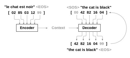
The goal is to construct a chatbot by utilizing a Sequence-to-Sequence (Seq2Seq) model, which encompasses both an encoder and a decoder, allowing it to process variable-length inputs and generate variable-length outputs.

Solution

The Seq2Seq model, often applied in machine translation, question-answering systems, and chatbots, is composed of two major components: an encoder and a decoder.

1. Encoder

   The encoder maps the input sequence $X = (x_1, x_2, \dots, x_T)$ to a fixed-dimensional context vector $C$. Each $x_t$ represents an element of the sequence (e.g., a word or a token). The context vector is then passed to the decoder.

   Mathematically, the forward pass of the encoder for each time step is as follows:

   \[h_t = \text{RNN}(x_t, h_{t-1})\]

   Here, $h_t$ is the hidden state at time step $t$, and it captures information from all the previous time steps.

   The final hidden state, $h_T$, serves as the context vector $C$.

2. Decoder

   The decoder, initialized with the context vector $C$, generates the output sequence $Y = (y_1, y_2, \dots, y_{T’})$. Unlike the input sequence, the output sequence can have a different length.

   At each time step, the decoder utilizes the context vector and its own hidden state to make a prediction.

   Mathematically, the forward pass of the decoder is as follows:

   \[\begin{aligned} s_0 &= f(h_T) \\ s_t &= \text{RNN}(y_{t-1}, s_{t-1}, c) \\ p(y_t | y_{t-1}, \dots, y_1, C) &= \text{softmax}(\text{FC}(y_{t-1}, s_t, c)) \end{aligned}\]

   Here, $s_t$ is the hidden state of the decoder at time step $t$, and $p(y_t

   y_{t-1}, \dots, y_1, C)$ is the probability distribution of the next token in the output sequence.

3. Training

   During training, the model strives to minimize the cross-entropy loss between the predicted and actual sequences.

Sequence-to-Sequence (Seq2Seq) Model

Implementation

Here is the Python PyTorch code for a basic Seq2Seq model:

import torch
import torch.nn as nn

class Encoder(nn.Module):
    def __init__(self, input_dim, emb_dim, hidden_dim, n_layers, dropout):
        super().__init__()
        self.hidden_dim = hidden_dim
        self.n_layers = n_layers
        self.embedding = nn.Embedding(input_dim, emb_dim)
        self.rnn = nn.GRU(emb_dim, hidden_dim, n_layers, dropout=dropout)

    def forward(self, src):
        embedded = self.embedding(src)
        outputs, hidden = self.rnn(embedded)
        return hidden

class Decoder(nn.Module):
    def __init__(self, output_dim, emb_dim, hidden_dim, n_layers, dropout):
        super().__init__()
        self.output_dim = output_dim
        self.hidden_dim = hidden_dim
        self.n_layers = n_layers
        self.embedding = nn.Embedding(output_dim, emb_dim)
        self.rnn = nn.GRU(emb_dim, hidden_dim, n_layers, dropout=dropout)
        self.fc_out = nn.Linear(hidden_dim, output_dim)

    def forward(self, input, hidden):
        input = input.unsqueeze(0)
        embedded = self.embedding(input)
        output, hidden = self.rnn(embedded, hidden)
        prediction = self.fc_out(output.squeeze(0))
        return prediction, hidden

class Seq2Seq(nn.Module):
    def __init__(self, encoder, decoder, device):
        super().__init__()
        self.encoder = encoder
        self.decoder = decoder
        self.device = device

    def forward(self, src, trg, teacher_forcing_ratio=0.5):
        batch_size = trg.shape[1]
        trg_len = trg.shape[0]
        trg_vocab_size = self.decoder.output_dim
        outputs = torch.zeros(trg_len, batch_size, trg_vocab_size).to(self.device)
        hidden = self.encoder(src)
        input = trg[0, :]
        for t in range(1, trg_len):
            output, hidden = self.decoder(input, hidden)
            outputs[t] = output
            teacher_force = random.random() < teacher_forcing_ratio
            top1 = output.max(1)[1]
            input = trg[t] if teacher_force else top1
        return outputs

58. Code a ResNet in Keras and train it on a dataset with transfer learning.

Problem Statement

The goal is to implement a ResNet-50 architecture in Keras for transfer learning on a dataset.

Solution

Implementing a ResNet-50 architecture and training it on a custom dataset using transfer learning involves the following steps:

1. Load the Data: Prepare the dataset and divide it into training and validation sets.

2. Create the Model: Define the ResNet-50 model architecture, optionally loading weights pre-trained on ImageNet.

3. Compile the Model: Set the loss function, optimizer, and evaluation metrics.

4. Train the Model: Use the fit function while monitoring performance on the validation set.

5. Evaluate the Model: Analyze its performance on the test set.

Implementation

Here is the Python code:

from keras.applications import ResNet50
from keras.models import Model
from keras.layers import Dense, GlobalAveragePooling2D
from keras.optimizers import Adam
from keras.preprocessing.image import ImageDataGenerator

# Set constants
num_classes = 10
img_width, img_height = 224, 224
batch_size = 32

# Load the ResNet50 base model
base_model = ResNet50(weights='imagenet', include_top=False, input_shape=(img_width, img_height, 3))

# Freeze the base model layers
for layer in base_model.layers:
    layer.trainable = False

# Add custom classification layers
x = base_model.output
x = GlobalAveragePooling2D()(x)
x = Dense(1024, activation='relu')(x)
predictions = Dense(num_classes, activation='softmax')(x)
model = Model(inputs=base_model.input, outputs=predictions)

# Compile the model
model.compile(optimizer=Adam(lr=0.0001), loss='categorical_crossentropy', metrics=['accuracy'])

# Data Augmentation and Loading
train_datagen = ImageDataGenerator(
    rescale=1./255,
    shear_range=0.2,
    zoom_range=0.2,
    horizontal_flip=True)

test_datagen = ImageDataGenerator(rescale=1./255)

train_generator = train_datagen.flow_from_directory(
    'data/train',
    target_size=(img_width, img_height),
    batch_size=batch_size,
    class_mode='categorical')

validation_generator = test_datagen.flow_from_directory(
    'data/validation',
    target_size=(img_width, img_height),
    batch_size=batch_size,
    class_mode='categorical')

# Train the model
model.fit_generator(
    train_generator,
    steps_per_epoch=train_generator.samples // batch_size,
    epochs=10,
    validation_data=validation_generator,
    validation_steps=validation_generator.samples // batch_size)

# Save the model
model.save('resnet50_trained_model.h5')

# Evaluate the model
test_generator = test_datagen.flow_from_directory(
    'data/test',
    target_size=(img_width, img_height),
    batch_size=batch_size,
    class_mode='categorical',
    shuffle=False)

loss, accuracy = model.evaluate_generator(
    test_generator,
    steps=test_generator.samples // batch_size)

print(f'Test accuracy: {accuracy*100:.2f}%')

This code is an entry point for training a ResNet-50 model using Keras.

59. Implement a Transformer model for a language translation task.

Problem Statement

The task is to implement a Transformer model for language translation, which is a popular application of deep learning in natural language processing (NLP).

Solution

Transformer architecture was introduced in the paper “Attention is All You Need” by Vaswani et al. It aims to handle sequential data, like sentences, more efficiently than previous models that leveraged recurrent or convolutional layers. The Transformer model benefits from parallelization due to its self-attention mechanism.

Architecture Components

• Embedding Layer: Transforms words to fixed-size vectors.
• Positional Encoding: Provides position-based information to the model.
• Encoder and Decoder Stacks: Composed of multiple identical layers. Each layer has two main sub-layers: Multi-Head Self-Attention mechanism and a simple, position-wise fully connected feed-forward network. It also leverages Residual connections and Layer Normalization.

The Self-Attention Mechanism

In the self-attention mechanism, for each word, the model assigns importance (attention weights) to all the other words in the sentence.

Multi-Head Self-Attention is performed in parallel for several different (Q, K, V) (Query, Key, Value) representations of the input. This enables the model to focus on different parts of the sentence based on different relationships learned during training.

Position-wise Feed-Forward Networks

After the Self-Attention mechanism, the model applies a two-layer position-wise feed-forward network to each position independently and identically. This greatly enhances the model’s representation power.

Positional Encoding

As the model doesn’t have a built-in understanding of the order of the elements in the sequence, positional encodings are added to the input embeddings. Sinusoidal functions are commonly used to encode this positional information.

Decoder’s Masked Self-Attention

While the encoder processes the entire input sequence at once, the decoder is designed to be autoregressive, meaning it generates one word at a time while attending to the previously generated words.

This requires a masked self-attention mechanism to be used in the decoder’s layers, which ensure that the word being generated cannot attend to future words.

Additional Details

• Model Variants: Transformer is the base model, while BERT, GPT, and T5 are popular variants, each optimized for different tasks.
• Implementation: PyTorch or TensorFlow/Keras can be used to implement the algorithm.

Performance Considerations

• Training Time: Transformers are efficient due to parallelization.
• Inference Time: Enhanced with the use of dynamic programming-based algorithms for beam search or sequence generation.
• Scalability: Proven to work well on both small and large datasets.

Limitations

Despite its advantages, Transformer models can suffer from high memory requirements, especially for long sequences or large batch sizes. Techniques such as pruning and quantization are often employed to address these issues.

Experimentation

When implementing the transformer model, it is crucial to experiment with various hyperparameters, including the number of layers, attention heads, and feed-forward dimensions, to identify the configuration that best fits the specific dataset and task.

60. Create an anomaly detection system using an autoencoder.

Problem Statement

The task is to detect anomalies (outliers) in data using an Autoencoder, a type of neural network extensively utilized for unsupervised learning.

Solution

Autoencoders consist of an encoder, which compresses the input, and a decoder, which attempts to reconstruct the original input. In the case of anomaly detection, the model is trained on ‘normal’ data and seeks to minimize the reconstruction loss. Anomalies are instances that the model struggles to reconstruct accurately.

Architecture

The most commonly used autoencoders for anomaly detection are the denoising autoencoder (DAE) and the variational autoencoder (VAE). In this context, we will focus on a simple DAE.

A basic autoencoder architecture consists of an input layer, a hidden layer (representing the compressed data), and an output layer.

Loss Function

The loss function for anomaly detection is typically the mean squared error (MSE) between the input and the reconstruction. A higher MSE indicates that the input is less representative of the learned ‘normal’ data.

This loss function is constructed to signal anomalies as deviations from the norm.

Regularization

Adding noise to the input data during training (hence ‘denoising autoencoder’) can improve the model’s ability to reconstruct normal patterns, enhancing its sensitivity to anomalies.

Training

• Normal Data Selection: Initially, only ‘normal’ or non-anomalous data should be used for training.
• Model Evaluation: After training, the model’s performance is validated on a separate dataset. Instances with high reconstruction loss are identified as potential anomalies.

Implementation

Here is a Python code to create the DAE model:

import numpy as np
import tensorflow as tf
from tensorflow import keras
from tensorflow.keras import layers

# Create an instance of the Sequential API
model = keras.Sequential()

# Add a denoising autoencoder layer
model.add(layers.Dense(128, activation='relu', input_shape=(n_features,)))
model.add(layers.GaussianNoise(0.1))  # Gaussian noise for regularization
model.add(layers.Dense(n_features, activation='sigmoid'))  # Sigmoid to scale values between 0 and 1

# Compile the model
model.compile(optimizer='adam', loss='mean_squared_error')

# Train the model
model.fit(X_train, X_train, epochs=50, batch_size=128, validation_data=(X_val, X_val))

---

Part 3 of the 80 Essential Deep Learning Interview Questions series. Next: Part 4: Applied Deep Learning & System Design (Q61-80).