80 Essential Deep Learning Interview Questions (21-40)

This is Part 2 of a 4-part series covering 80 essential deep learning interview questions. Questions 21–40 focus on loss functions, optimization, regularization, and training stability.

Study tip: For optimization questions, be ready to explain why Adam typically outperforms SGD early in training, and when SGD+momentum beats Adam for final convergence.

---

📉 21. What are loss functions, and why are they important?

A loss function (or cost function) is a critical part of training a machine learning model. Loss functions measure the performance of a model for given input data and the corresponding output, allowing the optimization algorithm to update the model’s parameters efficiently.

Key Components of a Loss Function

• True Values: The ground-truth data against which a model’s predictions are compared.
• Predicted Values: Output generated by the model for a given input.
• Error Measurement: The method for quantifying the discrepancy between the predicted and true values.

Types of Loss Functions

• Regression Loss Functions: Tailored for tasks where the goal is to predict continuous outcomes such as temperature, sales revenue, or stock prices.
• Classification Loss Functions: Designed for predicting discrete categories, typical in tasks like spam filtering (binary classification) or image recognition (multi-class classification).

Regression Loss Functions

• \textbf{Mean Absolute Error (MAE)}: Calculates the absolute differences between the predicted and true values and then computes their mean. This measure treats all differences equally.

  $$\text{MAE} = \frac{1}{n} \sum_{i=1}^{n} | y_i - \hat{y}_i |$$

• \textbf{Mean Squared Error (MSE)}: Squares the differences between predicted and true values before averaging them. The squaring gives more significant weight to larger errors.

  $$\text{MSE} = \frac{1}{n} \sum_{i=1}^{n} (y_i - \hat{y}_i)^2$$

• \textbf{Root Mean Squared Error (RMSE)}: The square root of MSE. It’s in the same units as the data and easier to interpret.

  $$\text{RMSE} = \sqrt{\text{MSE}}$$

• \textbf{Huber Loss}: A hybrid of MAE and MSE, which uses a “delta” parameter to switch between the two. It behaves like MAE when the error is small and like MSE when it’s large. This makes it less sensitive to outliers than MSE.

  $$L_{\delta}(x) = \begin{cases} \frac{1}{2}x^2 & \text{for } |x| \leq \delta \\ \delta(|x| - \frac{1}{2}\delta) & \text{otherwise} \end{cases}$$

• • Quantile Loss:
  • Mean Squared Logarithmic Error (MSLE): Computes the logarithm of the predictions and true values before computing the error. This loss metric is useful when the target values are skewed or when relative errors are more meaningful than absolute errors.
  • Cosine Embedding Loss: Specifically useful when dealing with problems that can benefit from measuring similarities.
• • Multimodal Discrepancy Loss: Purpose-built for multimodal distributions in the target variable.

Classification Loss Functions

Commonly-used loss functions for different types of classification tasks:

• Binary Classification:

  • Binary Cross-Entropy Loss (Log Loss): Binary classification tasks, where predictions are either 0 or 1.
  • Sigmoid Cross-Entropy Loss: This is similar to Binary Cross-Entropy Loss but uses the sigmoid activation function explicitly.
  • Hinge Loss: Especially useful for models involving support vector machines (SVMs).

• Multi-Class Classification:

  • Categorical Cross-Entropy Loss: Suitable for multi-class tasks, where predictions are divided into categorical classes. This loss function computes the entropy between the true and predicted distributions.
  • Sparse Categorical Cross-Entropy Loss: Similar to Categorical Cross-Entropy, but the true labels are not one-hot encoded, which makes it more memory-efficient.

• Multi-Label Classification:

  • Sigmoid Cross-Entropy Loss: Well-suited for multi-label tasks, where each input can belong to multiple labels or classes. This function uses the sigmoid activation to convert real-valued predictions to the range [0, 1].

When to Use Custom Loss Functions

Standard loss functions are effective in many scenarios, but there are also times when a custom loss function may be necessary, such as when the loss generated by the model doesn’t fit into any pre-existing loss function categories or if the task at hand is unique.

A custom loss function can help the machine learning model in understanding the complexities of the data. For instance, in cases where the metric of interest is not optimally represented by the existing loss functions.

Practical Considerations for Choosing a Loss Function

• Task Relevance: Select a loss function most appropriate for your specific machine learning task.
• Metric Alignment: It’s often beneficial to choose a loss function aligned with the evaluation metric you plan to use.
• Model Behavior: Some loss functions steer the model in specific directions, so understanding their impact on training is crucial.
• Data Characteristics: Sensitivity to outliers, target data distribution, and class imbalances are key considerations.

Implementing Custom Loss Functions in TensorFlow

Here is an example code:

import tensorflow as tf

# Custom Huber loss function
def huber_loss(y_true, y_pred):
    error = y_true - y_pred
    is_small_error = tf.abs(error) <= 1
    small_error_loss = tf.square(error) / 2
    large_error_loss = (1 - is_small_error) * (tf.abs(error) - 0.5)
    return tf.reduce_mean(tf.where(is_small_error, small_error_loss, large_error_loss))

# Compiling the model with custom loss function
model.compile(optimizer='adam', loss=huber_loss, metrics=['mae'])

# Fitting the model
model.fit(x_train, y_train, epochs=10, batch_size=32, validation_data=(x_val, y_val))

22. Explain the concept of gradient descent.

Gradient Descent is the cornerstone of many optimization algorithms in machine learning, particularly for refining the weights and biases within neural networks.

It’s a method for minimizing the loss function of a model by iteratively adjusting its parameters in the direction opposite to the estimated gradient.

Core Steps in Gradient Descent

1. Initialize Parameters: Start with an initial guess for the model’s parameters, referred to as weights and biases in neural networks.

2. Compute Gradient: Calculate the partial derivatives of the loss function with respect to each parameter to determine the slope.

3. Update Parameters: Modify the parameters (weights and biases) in the opposite direction of the gradient to decrease the loss.

4. Convergence Check: Verify if a termination criterion is met, such as a maximum number of iterations or a small change in the loss.

5. Output: The optimized parameters provide the best-fit model.

Coursera provides a very helpful explanation and mathematical breakdown of optimizing an objective function using gradient descent through the minimization problem for a parabolic curve in their lecture on the “Optimizing a Cost Function - Gradient Descent””>

Using code will make it more concrete. Here is the Python code:

# Import the library
import numpy as np

# Initialize the parameters
learning_rate = 0.01
num_iterations = 100
weights = [1.5, 0.5]

# Define the data and the model
X = np.array([1, 2, 3, 4, 5])
y = np.array([2, 3, 3.5, 5, 6.5])
def model(x, w): # w represents weights
    return w[0] * x + w[1]

# Define the loss function
def loss(y_true, y_pred):
    return np.mean(np.square(y_true - y_pred))

# Implement Gradient Descent
for _ in range(num_iterations):
    # Predict using the current model
    y_pred = model(X, weights)
    
    # Compute the gradient
    gradient = [-2 * np.mean((y - y_pred) * X), -2 * np.mean(y - y_pred)]
    
    # Update weights
    weights = [w - learning_rate * g for w, g in zip(weights, gradient)]
    
    # Calculate and monitor the loss
    current_loss = loss(y, y_pred)
    print(f"Iteration: {_+1}, Loss: {current_loss}, Weights: {weights}")

23. What are the differences between batch gradient descent, stochastic gradient descent, and mini-batch gradient descent?

Gradient Descent is an iterative optimization algorithm used to minimize a loss function, especially in the context of training Deep Learning models. The three main variations of the algorithm are Batch, Stochastic, and Mini-Batch Gradient Descent.

Core Differences

Batch Gradient Descent

In Batch Gradient Descent, the model parameter updates are determined using the gradients calculated across the entire dataset.

Key Points:

• Robustness: Requires full dataset for each iteration; can be computationally expensive.
• Convergence: Smooth, consistent updates help in converging to the true minima rather than settling for local minima, especially in convex problems. More stable convergence in deep, non-convex problems.
• Parallelization: Does not benefit from parallel computing as it depends on the full dataset.

Stochastic Gradient Descent

In Stochastic Gradient Descent, the model parameters are updated after each individual training example is presented.

Key Points:

• Robustness: Potentially noisy and erratic due to frequent updates, but generally converges faster, benefiting from the immediate local information in each sample.
• Convergence: The “noisiness” in the direction of the gradient can cause oscillations. However, this keeps the algorithm from getting stuck in local minima, especially in non-convex optimization landscapes.

Mini-Batch Gradient Descent

Mini-Batch Gradient Descent operates as a balance between the previous two methods, taking an update step after processing a small subset or batch of the training dataset.

Key Points:

• Trade-Off: Combines efficiency of calculations over a set of examples (useful for modern hardware or distributed environments) with the potential robustness benefits from stochastic updates.
• Adaptability: Often used as a default, especially for problems involving larger datasets.

Code Example: Variants of Gradient Descent

Here is the Python code:

# Batch Gradient Descent
def batch_gradient_descent(model, X, y, learning_rate, num_epochs):
    m = len(y)
    for epoch in range(num_epochs):
        loss = model.compute_loss(X, y)
        gradients = model.compute_gradients(X, y)
        model.update_parameters(gradients, learning_rate)

# Stochastic Gradient Descent
def stochastic_gradient_descent(model, X, y, learning_rate, num_epochs):
    for epoch in range(num_epochs):
        for i in range(len(y)):
            loss = model.compute_loss(X[i], y[i])
            gradients = model.compute_gradients(X[i], y[i])
            model.update_parameters(gradients, learning_rate)

# Mini-Batch Gradient Descent
def mini_batch_gradient_descent(model, X, y, learning_rate, batch_size, num_epochs):
    m = len(y)
    num_batches = int(m / batch_size)
    
    for epoch in range(num_epochs):
        shuffled_indices = np.random.permutation(m)
        X_shuffled, y_shuffled = X[shuffled_indices], y[shuffled_indices]
        for batch in range(num_batches):
            start, end = batch * batch_size, (batch + 1) * batch_size
            X_batch, y_batch = X_shuffled[start:end], y_shuffled[start:end]
            loss = model.compute_loss(X_batch, y_batch)
            gradients = model.compute_gradients(X_batch, y_batch)
            model.update_parameters(gradients, learning_rate)

24. Discuss the role of learning rate in model training and its impact.

Learning rate is a crucial hyperparameter in training machine and deep learning models. It determines the size of the step that a model takes while optimizing its parameters using techniques like gradient descent.

Learning Rate Mechanism

At each iteration, gradient descent adjusts model parameters based on the magnitude and sign of the gradient. The learning rate, denoted as α \alpha , scales this adjustment.

The update formula for a parameter θ \theta is:

θ=θ−α⋅∇J(θ) \theta = \theta - \alpha \cdot \nabla J(\theta)

Where ∇J(θ) \nabla J(\theta) represents the gradient of the cost function J J with respect to θ \theta . The learning rate, in essence, controls the convergence speed and stability of the optimization process.

Tuning the Learning Rate

Selecting the appropriate learning rate is essential for effective model training. An ideal learning rate generally:

• Allows for convergence during training.
• Results in stable, oscillation-free learning.
• Achieves a good compromise between speed and accuracy, aiming for the optimal minimum.

Impact of Learning Rate

Overshooting

• Too High: The model might overshoot the minimum, causing it to diverge or oscillate around the minimum.

Slow Convergence

• Too Low: The model might take an excessive number of iterations to converge or get stuck in a local minimum.

Fine-Tuning the Goldilocks Learning Rate

• Using grid search or algorithms like cyclical learning rates can help to narrow down the ideal range and value for the learning rate.

Visualising the Learning Rate’s Impact

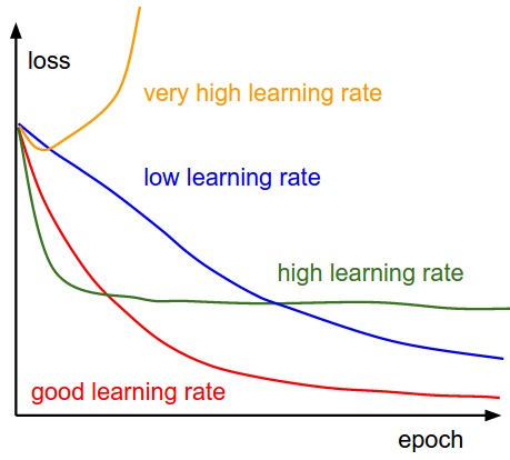
Adaptive Learning Rates

To alleviate the need for manual tuning, techniques like Adagrad, RMSprop, and Adam dynamically adjust the learning rate based on past gradients. Such adaptive learning rate methods can often converge faster and more reliably than fixed learning rates.

25. What are optimization algorithms like Adam, RMSprop, and AdaGrad?

Adam, RMSprop, and AdaGrad are three key optimization algorithms within the realm of stochastic gradient descent. They are specifically designed to manage issues often encountered when optimizing deep learning models.

Core Concepts

Gradient Descent as a Foundation

Both traditional gradient descent and its stochastic counterpart involve iteratively adjusting model parameters to minimize a cost function.

Stochastic gradient descent is a popular choice in deep learning for its speed and scalability. However, it can be erratic due to its noisy gradients.

Managing Gradients

Advanced optimization mechanisms tackle gradient noise. They tame huge gradients, typical in the initial stages, and enable continued learning from the data as the model gets refined.

Albert Einstein’s feature selection paper gives the basic idea behind stochastic gradient descent.

Adaptive Learning Rate

A key aspect of these advanced optimization methods is an adaptive learning rate. Unlike standard gradient descent, where the learning rate is global and static during the training process across all model parameters, these algorithms offer unique learning rate values for each parameter of the model.

This adaptability ensures smoother and faster convergence, aligning the algorithms with the characteristics of the individual parameters they influence in the most effective manner.

Algorithm Structures

RMSprop

RMSprop is designed to tackle two adverse situations that can arise as a neural network model progresses in its training:

1. The Learning Rate: It tends to decrease to a level where it fails to make any meaningful adjustments to model parameters.
2. Sparse Gradients: For relatively infrequently occurring features, the gradients can be sparse, making efficient optimization challenging.

To address these, the algorithm maintains an exponentially decaying average of past squared gradients, tailored to each parameter. Dividing the current gradient by the square root of this average ensures a more appropriate learning rate for that specific parameter.

Code Example: RMSprop

Here is the Python code:

# Initialize parameters
learning_rate = 0.01
epsilon = 1e-8
decay_rate = 0.9
cache = np.zeros_like(parameters)

# Update parameters
cache = decay_rate * cache + (1 - decay_rate) * (grad ** 2)
parameters -= learning_rate * grad / (np.sqrt(cache) + epsilon)

Adam

Adam, short for adaptive moment estimation, combines features from RMSprop and momentum, which is effective in overcoming local minima in the cost function.

In addition to utilizing past squared gradients like RMSprop, it also keeps track of exponentially decaying averages of past gradients, incorporating a “momentum” effect.

The algorithm integrates this adaptive learning rate and momentum, ensuring an efficient balance during parameter updates.

Code Example: Adam

Here is the Python code:

# Initialize parameters
alpha = 0.001
beta1 = 0.9
beta2 = 0.999
epsilon = 1e-8

# Update parameters
grad_squared = grad ** 2
m = beta1 * m + (1 - beta1) * grad
v = beta2 * v + (1 - beta2) * grad_squared
m_hat = m / (1 - beta1)
v_hat = v / (1 - beta2)
parameters -= alpha * m_hat / (np.sqrt(v_hat) + epsilon)

AdaGrad

AdaGrad, or adaptive gradient algorithm, is exceptionally effective with sparse data. Its standout feature is that it modifies the learning rate globally for every model parameter based on the magnitude of its associated gradients.

It accomplishes this by accumulating the squares of gradients during training and then using a divisor consisting of the square root of this accumulation to rescale the learning rate.

However, for cases where sparse gradients are not desirable, it may potentially lock in parameters.

Code Example: AdaGrad

Here is the Python code:

# Initialize parameters
alpha = 0.01
epsilon = 1e-8
grad_squared_sum = 0

# Update parameters
grad_squared_sum += grad ** 2
parameters -= (alpha / (np.sqrt(grad_squared_sum) + epsilon)) * grad

Selecting the Right Algorithm

Adam, RMSprop, and AdaGrad, all provide adaptive learning rates, which can prevent the learning rate from becoming excessively large. For dense data, Adam typically achieves the most consistent results. For scenarios involving sparse gradients, RMSprop has proven advantages. If learning from sparse data is the primary focus, then AdaGrad may be the most suitable choice.

26. How does _Batch Normalization work?

Batch Normalization (BN) is a technique to improve the speed, stability, and performance of deep learning models. It standardizes the activations of each layer to have zero mean and unit variance using mini-batches of data during training.

The process has a number of benefits, such as reducing the effects of vanishing or exploding gradients, which in turn allows for the use of higher learning rates, leading to faster convergence.

Mean and Variance Adjustment

For each mini-batch, BN adjusts the mean and variance of each layer, ensuring all features have the same scale. This is crucial for enabling gradient descent to work effectively.

The adjusted values $\mu_B$ and $\sigma_B^2$ for a mini-batch can be computed as:

\[\begin{aligned} \mu_B &= \frac{1}{m} \sum_{i=1}^{m} x_i \\ \sigma_B^2 &= \frac{1}{m} \sum_{i=1}^{m} (x_i - \mu_B)^2 \end{aligned}\]

Where:

• $m$ is the batch size
• $x_i$ are the input activations

Normalization and Rescaling

Once the mean and variance are obtained for each mini-batch, the inputs are normalized using this formula:

\[\hat{x}_i = \frac{x_i - \mu_B}{\sqrt{\sigma_B^2 + \epsilon}}\]

Where:

• $\epsilon$ is a small positive number for numerical stability

The normalized activations are then rescaled and shifted using the learned scaling factor $\gamma$ and shift factor $\beta$ for each layer:

\[y_i = \gamma \hat{x}_i + \beta\]

Cross-Batch Mean and Variance Propagation

During inference, the model might receive inputs or data points one at a time, sans any mini-batch structure. In such cases, BN uses estimated values from the training data to normalize and scale.

For each layer, BN maintains two additional sets of parameters $(\mu, \sigma^2)$ , which can be thought of as running averages across the different mini-batches during training. These parameters provide an estimate of the mean and variance for the entire dataset.

The Role of Momentum

To improve estimation quality, BN uses a momentum term typically set to 0.9 or similar. This term allows the running averages to evolve more slowly. The new mean and variance are computed as a weighted average between the current mini-batch values and the running estimate:

\[\begin{aligned} \mu &\leftarrow (1 - \text{momentum}) \times \mu + \text{momentum} \times \mu_B \\ \sigma^2 &\leftarrow (1 - \text{momentum}) \times \sigma^2 + \text{momentum} \times \sigma_B^2 \end{aligned}\]

Code Example: Batch Normalization

Here is the Python code:

import numpy as np

# Input data
X = np.array([[1, 2, 3],
              [4, 5, 6]])

# Assume mean and variance for illustration
mean, var = 2.5, 2.92

# Calculate normalized activations
batch_normalized = (X - mean) / np.sqrt(var + 1e-8)

# Assume BN parameters
gamma, beta = 1.5, 0.5

# Rescale and shift
y = gamma * batch_normalized + beta

In a more comprehensive scenario, these steps would be integrated into the training algorithm and would involve multiple layers and mini-batches of data.

27. Describe the process of hyperparameter tuning in neural networks.

Hyperparameter tuning is essential to optimize neural network models. This process, also known as hyperparameter optimization, involves systematically searching through different hyperparameter combinations to identify the set that yields the best performance.

Steps in Hyperparameter Tuning

1. Define Hyperparameters: This involves selecting the hyperparameters that define the architecture of the neural network, as well as the training process.

2. Choose a Strategy for Optimization: Methods range from grid search and random search to more advanced techniques like Bayesian optimization or evolutionary algorithms.

3. Set Evaluation Metrics: Select the primary metrics that define the success of your model.

4. Split Data for Validation: Divide your dataset into training, validation, and test sets. Cross-validation can be used in place of simple train-test splits for more robust evaluation.

Techniques for Hyperparameter Tuning

Baseline Estimation

Calculate performance of the model with default settings. This will give an understanding of accuracy of the model in raw state.

Grid Search

This method exhaustively searches through a pre-defined subset of hyperparameters. It’s computationally expensive but guarantees to find the best combination within the specified parameter space.

Random Search

Random search selects hyperparameter combinations at random from a pre-defined search space. It is computationally less demanding than grid search and often more effective.

Bayesian Optimization

This probabilistic model encodes a prior belief about the hyperparameters and updates it as new observations are made. Bayesian optimization targets the most promising hyperparameter combinations. It is particularly effective in optimizing time-intensive tasks.

Automated Hyperparameter Tuning Services

Many cloud-based machine learning platforms provide tools for automatic hyperparameter tuning. These services often use advanced algorithms and distributed computing to efficiently explore and optimize the hyperparameter space.

Tools and Libraries for Hyperparameter Tuning

• scikit-learn: Offers grid and random search via the GridSearchCV and RandomizedSearchCV classes.
• TensorFlow: The Keras tuner module provides tools for hyperparameter optimization.
• Hyperopt: A flexible and versatile library for Bayesian optimization.

Code Example: Hyperparameter Optimization with Keras

Here is a Python code snippet:

import tensorflow as tf
from tensorflow import keras
from kerastuner.tuners import RandomSearch
from tensorflow.keras.layers import Dense

# Load the dataset, define hyperparameters, and select evaluation metrics

# Define the model-building function
def build_model(hp):
    model = keras.Sequential()
    model.add(Dense(units=hp.Int('units', min_value=32, max_value=512, step=32), activation='relu'))
    model.add(Dense(1, activation='sigmoid'))
    model.compile(optimizer='adam', loss='binary_crossentropy', metrics=['accuracy'])
    return model

# Initialize the hyperparameter tuner
tuner = RandomSearch(build_model, objective='val_accuracy', max_trials=5, executions_per_trial=3, directory='my_dir', project_name='helloworld')

# Start the hyperparameter search
tuner.search(x=train_dataset, y=train_labels, epochs=5, validation_data=(val_dataset, val_labels))

# Retrieve the best model
best_model = tuner.get_best_models(num_models=1)[0]

28. What is early stopping, and how does it prevent overfitting?

Early stopping involves halting the training process of a model when its performance on a validation dataset starts to degrade. This technique is used to counteract overfitting in deep learning and other machine learning methods.

Overfitting: A Brief Overview

• Overfitting occurs when a model learns the training data too well, to the point that it impairs its ability to generalize to new, unseen data.
• In this scenario, the model has high accuracy on the training dataset but performs significantly less accurately on validation or test sets.

Visual Representation of Overfitting

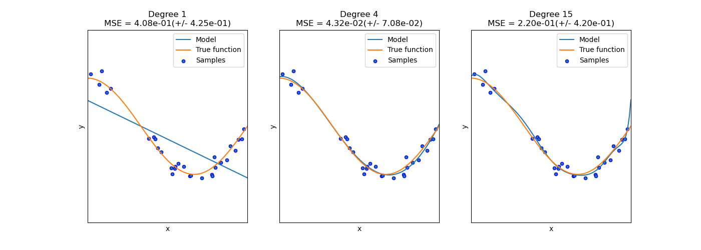
Understanding Overfitting and Early Stopping

1. Loss Function: When we train models, we often have an associated loss function. For instance, in a classification task, we would use a cross-entropy loss. This loss is directly linked to the model’s predictive performance.

   • Training Loss: The loss computed on the data the model is being trained on.
   • Validation Loss: The loss computed on a separate dataset, the validation set, which wasn’t used for training.

2. Optimization Algorithm: In most neural network setups, we use an iterative optimization algorithm, such as stochastic gradient descent (SGD). This algorithm aims to minimize the loss function.

3. Validation Loss as an Early-Stopping Criterion: During the model training, monitoring the validation loss gives us an indication of how well the model is doing on unseen data.

Code Example: Early Stopping with Keras

Here is the Python Keras code:

from tensorflow.keras.models import Sequential
from tensorflow.keras.layers import Dense
from tensorflow.keras.callbacks import EarlyStopping

# Some data, X_train, X_val, y_train, y_val

# Initialize the model
model = Sequential()
model.add(Dense(32, input_dim=10, activation='relu'))
model.add(Dense(1, activation='sigmoid'))

# Compile the model
model.compile(optimizer='adam', loss='binary_crossentropy', metrics=['accuracy'])

# Initialize early stopping
early_stopping = EarlyStopping(monitor='val_loss', patience=5)

# Train the model
model.fit(X_train, y_train, validation_data=(X_val, y_val), epochs=100, callbacks=[early_stopping])

In this example, we use Keras’s EarlyStopping callback. We set monitor='val_loss' to indicate we are monitoring the validation loss. The patience parameter is set to 5, meaning training will stop after 5 epochs of no improvement on the validation loss. This way, early stopping helps prevent overfitting.

Practical Considerations

• Training duration: Early stopping can significantly reduce the time required to train models, especially when accuracies stabilize quickly.
• Model checkpointing: It’s a common practice to combine early stopping with “model checkpointing,” which saves the best model observed so far. This ensures that the model returned is the one that performed the best in terms of validation loss.

Hyperparameter: Patience

The patience hyperparameter represents the number of epochs with no improvement after which training will be stopped. Setting patience too low can lead to premature stopping, whereas setting it too high might allow the model to overfit before stopping.

It is often set based on the data and the problem at hand, and cross-validation or a visual inspection of the learning curve can help determine an appropriate value.

Disadvantages of Early Stopping

• Limited Generalization: Halting training early means the model may not reach its full potential, possibly restricting its capabilities.
• Potential for Noise: If the validation dataset is small or noisy, early stopping decisions may be unreliable.

Alternatives to Early Stopping

• Data Augmentation: Techniques like flipping or rotating images can artificially boost the size of the training set, potentially reducing overfitting.
• Regularization Methods: L1 and L2 regularization, dropout, and batch normalization, among others, are aimed explicitly at reducing overfitting by limiting the model’s capacity to memorize noise in the training data.

Early Stopping Variations

• Batch Early Stopping: Assess the model’s performance at the end of each epoch rather than after each individual batch.

• Adaptive Early Stopping: Adjust the patience threshold throughout training based on the model’s performance, reducing the risk of stopping too early.

Summary:

• Early stopping can effectively combat overfitting by monitoring how well the model generalizes to unseen data.
• Key considerations include choosing the right hyperparameters such as patience and combining early stopping with other techniques like data augmentation and regularization for a robust model.

Remember the integrated approach: early stopping is a valuable tool but is most effective when used in combination with other techniques!

29. Explain the trade-off between bias and variance.

Bias and Variance represent two sources of predicative error in machine learning models. The interplay between both concepts is referred to as the Bias-Variance Tradeoff.

Simplifying the Tradeoff

• High Bias, Low Variance: Models make strong assumptions leading to possible oversimplification (underfitting), resulting in consistent but possibly inaccurate predictions across different datasets.

• Low Bias, High Variance: Models are complex and responsive to data leading to being tailored to specific datasets (overfitting), causing predictions to swing significantly between training and test data.

Finding the Middle Ground

The objective is to strike a balance between bias and variance. A good model generalizes well to unseen data.

• Sweet Spot: Models aim for both low bias (good fit in general) and low variance (stable predictions across different datasets).

Formalizing the Relationship

For a regression task with model parameter θ \theta and target variable Y Y :

Expected Loss=Bias2+Variance+Irreducible Error \text{Expected Loss} = \text{Bias}^2 + \text{Variance} + \text{Irreducible Error}

Here, the Irreducible Error is the noise in the data that cannot be reduced regardless of how accurate the model is.

Bias-Variance Interface

• As model complexity increases, bias generally decreases but variance can start to rise due to the model being sensitive to the specific training data.
• Increasing the dataset size can lower variance but will have little effect on the bias.

Practical Strategies

1. Cross-Validation: Assess model performance across multiple subsets of the data to better identify bias and variance.

2. Regularization: Penalize the model for being overly complex, helping control variance.

3. Feature Selection/Dimensionality Reduction: Simplify the model and reduce noise, curbing variance.

4. Ensemble Methods such as bagging, boosting, or model averaging: Combine predictions from multiple models to aim for lower variance and, ideally, lower bias as well.

30. How do you use transfer learning in deep learning?

Transfer learning is a technique in machine learning to leverage knowledge from one model to improve learning in another related task. In the context of deep learning, it involves using pre-trained neural networks as a foundation for different learning tasks.

Workflow

Implementing transfer learning typically follows these steps:

1. Select Pre-trained Model: Choose a neural network that performs well on a task similar to your target task.

2. Feature Extraction: Extract the learned representations (features) from the pre-trained model on the new dataset. This step can be either:

   • Fixed weights: The pre-trained layers’ weights remain constant, serving merely as feature extractors.
   • Fine-tuned weights: The weights of some or all layers can be updated to better fit the new dataset.

3. Adapt the Model’s Head: Replace the final layers of the pre-trained model with new ones tailored to your specific task, like classification or regression.

4. Train on Target Task: Train the adapted model on data specific to your task. Thanks to the initial knowledge from the pre-trained model, and often a shorter training time, you should achieve improved performance compared to training from scratch.

Code Example: Image Classification with Transfer Learning

Here is the Python code:

# Import necessary modules
from keras.applications import VGG16
from keras.models import Model
from keras.layers import Dense, Flatten, Dropout
from keras.optimizers import Adam
from keras.preprocessing.image import ImageDataGenerator

# Load pre-trained model with weights fixed
base_model = VGG16(weights='imagenet', include_top=False, input_shape=(224, 224, 3))

# Freeze weights of base model
for layer in base_model.layers:
    layer.trainable = False

# Define a custom top
x = Flatten()(base_model.output)
x = Dense(512, activation='relu')(x)
x = Dropout(0.5)(x)
predictions = Dense(20, activation='softmax')(x)

# Combine base model and custom top
model = Model(inputs=base_model.input, outputs=predictions)

# Compile the model
model.compile(Adam(lr=0.0001), loss='categorical_crossentropy', metrics=['accuracy'])

# Optional: Data Augmentation
train_datagen = ImageDataGenerator(rescale=1./255, shear_range=0.2, zoom_range=0.2, horizontal_flip=True)
test_datagen = ImageDataGenerator(rescale=1./255)

# Load and prepare training and validation data
train_data = train_datagen.flow_from_directory('path/to/train', target_size=(224, 224), batch_size=32, class_mode='categorical')
test_data = test_datagen.flow_from_directory('path/to/test', target_size=(224, 224), batch_size=32, class_mode='categorical')

# Train the model
model.fit_generator(train_data, steps_per_epoch=len(train_data), validation_data=test_data, validation_steps=len(test_data), epochs=10)

31. What are some popular libraries and frameworks for deep learning?

Here are some popular libraries and frameworks for deep learning:

TensorFlow

Developed by Google Brain in 2015, TensorFlow is an open-source library that supports both CPU and GPU computation and provides an intuitive computational graph visualizer, TensorBoard.

Keras

Keras, often used in conjunction with TensorFlow, is a high-level neural networks API. It allows for fast experimentation and provides a user-friendly interface for building neural networks.

PyTorch

Developed by Facebook, PyTorch is another open-source deep learning framework. It is known for its flexibility and dynamic computation graph, and it’s often chosen for research and rapid prototyping.

Theano

Pioneered by the Montreal Institute for Learning Algorithms (MILA) in 2007, Theano is a Python library that has been influential in shaping many deep learning libraries, such as Keras.

Caffe

Released in 2014 by the Berkeley Vision and Learning Center (BVLC), Caffe is a deep learning framework that is popular for its efficiency and scalability. It is often used in vision-related tasks.

Chainer

Developed by a team at Japanese IT company, Preferred Network, and released in 2015, Chainer is known for its flexibility and dynamic approach to neural network building.

MXNet

Backed by Apache, MXNet is an open-source deep learning framework that supports both symbolic and imperative programming. It is designed for distributed and multi-GPU computing.

Lasagne

A lightweight library based on Theano, Lasagne provides a simple API for constructing and training neural networks. Though no longer under active development, its methods have been incorporated into other libraries.

CNTK

Microsoft’s Cognitive Toolkit, typically abbreviated to CNTK, is an open-source deep learning framework. It is known for its efficiency and the ability to handle large datasets, as well as its support for multiple types of neural network structures.

DL4J

Short for Deeplearning4j, this is a distributed deep learning library for Java and Scala. It’s designed to be fast and scalable and can run on both CPUs and GPUs.

Mocha

Mocha.jl is a deep learning framework written in the Julia language. It boasts efficiency, and its development is spearheaded by members of the machine learning community associated with MIT.

PaddlePaddle

Released by Chinese internet company Baidu, PaddlePaddle is an open-source deep learning platform equipped with support for both static and dynamic computation graphs, as well as tools for federated learning.

Coffea

Coffea is a deep learning library written in the Crystal programming language. While it’s relatively new and less popular than others, it offers an efficient alternative for Crystal enthusiasts.

H2O.ai

Developed by the company H2O.ai, this open-source platform is designed for machine learning and deep learning tasks and is best known for its ML and AI capabilities.

MatConvNet

MatConvNet specializes in convolutional neural networks (CNNs) and is designed to intertwine seamlessly with MATLAB, making it a popular choice for MATLAB users.

Bob

The Bob framework offers a comprehensive suite of tools for various visual recognition tasks, especially in the biometrics and security domains, and integrates with other libraries like PyTorch and Keras.

DeepLearning.scala

With its roots in Scala, DeepLearning.scala leverages the language’s functional programming elements for deep learning tasks. It’s less mainstream than other libraries but may appeal to Scala enthusiasts.

MLPack

MLPack provides a broader spectrum of machine learning algorithms, including neural networks, with a focus on performance and ease of use. It’s written in C++ and is suitable for large-scale tasks.

Fractal.jl

Written in Julia, Fractal.jl is a newer multiplication and convolution library that focuses on utilizing hardware to achieve lightning-fast speeds while keeping a simple and accessible interface.

Lush

Lush is both a programming language and a library, designed to be a high-performance resource for neural network-related tasks. While not as widely known, it still has its dedicated user base.

OpenNN

OpenNN, short for “Open Neural Networks Library,” is an open-source library designed for research and real-world applications in the field of machine learning, especially deep learning.

Dlib

Although recognized as a C++ machine learning library, Dlib also incorporates various deep learning tools and has built-in support for tasks like object detection and image segmentation.

Accord.NET

Accord.NET is a combined machine learning and image processing framework for the .NET ecosystem. It integrates cutting-edge techniques and is frequently used for research and academic purposes.

LightGBM

Developed by Microsoft, LightGBM is a powerful, accurate, and efficient gradient boosting framework, which includes support for GPU-accelerated training.

CatBoost

Launched in 2017 by Russian search engine company Yandex, CatBoost is an open-source gradient boosting framework that’s optimized for categorical features in data.

XGBoost

XGBoost is a tried and tested gradient boosting library, known for its efficiency and performance and often used in winning solutions for machine learning competitions like Kaggle.

Hugging Face Transformers

Initially developed to optimize natural language processing models, Hugging Face Transformers now includes support for a wide range of tasks, including vision-related ones, and often integrates state-of-the-art models and architectures.

BigDL

From Intel AI Lab, BigDL is a distributed deep learning library for Apache Spark that leverages the deep learning ecosystem from various sources like TensorFlow and Keras.

RAPIDS

Created by NVIDIA, RAPIDS aims to bring GPU acceleration to both data processing and machine learning tasks, making use of cutting-edge tools and techniques for optimal performance.

TVM

TVM, or “Tensor Virtual Machine,” is a deep learning compiler stack designed to optimize deep learning computations for various types of hardware.

Owl

Owl is a numerical library that’s quite broad and robust, and while it’s not solely focused on deep learning, it does contain various neural network-related tools and methods for users.

TensorForce

TensorForce presents itself as a reinforcement learning library for TensorFlow and includes a wide range of algorithms out of the box, rooms for customization, and multi-agent systems support.

Akktor

Akktor is a relatively new arrival that focuses on bringing asynchronous deep learning to both CPUs and GPUs; it’s designed to facilitate seamless scaling as per computational requirements.

32. How can GPUs be utilized in training deep neural networks?

GPUs are invaluable in deep learning for their parallel processing capability. They can handle matrix operations and other tasks, which CPUs are generally less efficient at, thus significantly reducing training time.

Matrix Operations and Parallelism

• GPU: Uses thousands of cores in parallel to compute matrix operations quickly.
• CPU: Core optimization is more beneficial for general applications, providing strong single-core performance.

Benefits of GPU Parallelism

• Memory Bandwidth: Allows for faster access to data, crucial for deep learning workloads.
• Task Handling: Scales well with work that can be executed simultaneously.
• Overall Throughput: More cores can lead to more tasks processed in a given time frame.

Utilizing Both CPU and GPU

Modern machine learning libraries, such as TensorFlow and Keras, exploit the strengths of both CPUs and GPUs for more efficient computations.

Here is the Python code:

import tensorflow as tf

# Identify the available computing devices
physical_devices = tf.config.list_physical_devices('GPU')

# To limit memory usage in GPU
if physical_devices:
    try:
        tf.config.experimental.set_memory_growth(physical_devices[0], True)
    except RuntimeError as e:
        print(e)

# Make use of GPUs
with tf.device('/GPU:0'):
    # Model and data training setup here
    pass

# Use the CPU for other tasks
with tf.device('/CPU:0'):
    # Additional computations here
    pass

33. Explain how a deep learning model can be deployed into production.

Deploying a Deep Learning model for production involves several key steps to ensure its smooth and effective integration.

Steps for Deployment

1. Model Preparation: Fine-tune and optimize the model for efficient inference. For instance, you can use pruning, quantization, or distillation to reduce model size or complexity.

2. Inference Method: Select an appropriate method for model inference. It could involve real-time online inference, offline batch predictions, or an interactive mode.

3. Scalability and Efficiency: Ensure the model can handle production-level workloads. Utilize techniques like multi-threading, batch processing, and model parallelism to optimize performance.

4. Hardware Selection: Choose the most suitable hardware based on performance, cost, and power consumption requirements. Options range from CPUs and GPUs to specialized accelerators like TPUs.

5. Software Environment: Determine the software stack for model inference. For standard deep learning models, this typically involves a framework like TensorFlow, PyTorch, or Keras. For more specialized hardware or performance requirements, consider tools like TensorRT, OpenVINO, or TVM.

6. Middleware and Pipelines: Integrate the model into a middleware layer or a workflow pipeline that streamlines data input, pre-processing, model inference, and post-processing.

7. Monitoring and Maintenance: Establish mechanisms to continuously monitor the model’s performance in a production environment. This could include tracking inference latency, throughput, and accuracy, along with regular model retraining on updated data.

34. What are the considerations for scaling deep learning models?

Scaling deep learning models involves optimizing computational resources and designing networks to meet specific project requirements.

Key Considerations for Scaling

1. Data Set Size: More complex models require large datasets, often from the order of thousands of samples per feature.

2. Hardware and Memory: Deep Learning usually demands GPU acceleration for training, with memory requirements influenced by both the model size and the size of the training data.

3. Cross-Validation Times: Larger models or datasets can result in longer training times, potentially impeding efficient cross-validation.

4. Feature Engineering: While deep learning can automate some level of feature engineering, especially for raw data, it’s important to consider feature extraction and manipulation methods that can help decrease computational costs and potentially enhance model performance.

5. Statistical Power: Bigger models come with higher statistical power, which can uncover subtle patterns in data. However, discerning between meaningful and spurious associations can be challenging.

6. Model Complexity: Balancing the model’s capacity to fit the training data while preventing overfitting is crucial. In some scenarios, such as with vast datasets or straightforward, predictable patterns, simpler models might be more appropriate. Simpler models often require less computation, making them faster and less resource-intensive.

7. Underlying Algorithm: Tailoring the model and its parameters to match the scope of the project is essential. Using an algorithm adjusted to the dataset dimensions and the specifics of the task can boost computational efficiency and model effectiveness.

8. Training and Test Set Size Relationship: The training set size often guides the model’s capacity, while the test set size provides insights on the model’s performance. A balance is fundamental to avoid data leakage and statistical biases during model assessment.

9. Interpretability and Explainability: Increasing model size can potentially compromise interpretability and explainability. Depending on the context, there might be limitations on the upper bounds of model complexity.

10. Hyperparameter Optimisation: Larger models typically require more in-depth hyperparameter tuning, which can be computationally costly.

Techniques for Efficient Scaling

1. Transfer Learning: Tailoring a pre-trained model to a specific task reduces training time and data requirements.

2. Dimensionality Reduction: Techniques like PCA and LDA can help trim input dimensions, which can be particularly valuable in high-dimensional spaces.

3. Pruning and Quantization: Techniques like weight pruning and layer quantization reduce the model’s size, making it more efficient for inference.

4. Ensemble Methods: Combining outputs from multiple, often simpler, models can improve predictive power.

5. Online and Batch Learning: For continuous, fast-paced data, online or batch learning can be more effective than re-training the model from scratch.

6. Distributed Computing: Using multiple GPUs in parallel and distributing computations across nodes in a cluster can significantly speed up training.

35. What data preprocessing steps are important for training a deep learning model?

Successful data preprocessing is key to a deep learning model’s performance.

Data Preprocessing Steps

1. Data Collection:

   • Training/Validation/Test Split: Divide data into at least three sets.
   • Data Balance: Ensure balanced classes for better model performance.

2. Data Cleaning:

   • Missing Values: Address data points with missing components.
   • Outliers: Determine if outliers are genuine or errors, and handle them accordingly.
   • Noise Reduction: Eliminate irrelevant or redundant information that might hinder learning.

3. Feature Engineering and Selection:

4. Feature Scaling (Normalization/Standardization):

   • Scaling numerical features can enhance convergence and training speed of many models, especially ones using Gradient Descent.

5. Feature Encoding:

   • One-Hot Encoding: For categorical features and labels.
   • Label Encoding: For non-ordinal, categorical data.
   • Binary Encoding: For categorical data with high cardinality.

6. Input Reformatting:

   • Image Data: Reshape and normalize pixel values.
   • Text Data: Tokenization, padding, and potentially embedding or vectorizing methods.
   • Time Series Data: Reshape and standardize time series for compatibility.

7. Data Imbalance Resolution:

   • Techniques like undersampling, oversampling, and SMOTE can address class imbalances.

8. Handling Missing Data:

   • Techniques like mean/mode imputation or using algorithms that inherently handle such data (e.g., XGBoost) can be employed.

Keras Code Example: Basic Preprocessing Pipelines

Here is the Python code:

import numpy as np
from sklearn.model_selection import train_test_split
from sklearn.preprocessing import LabelEncoder, StandardScaler
from keras.utils import to_categorical

# Step 1: Data Collection & Basic Preprocessing
X, y = np.load('your_data.npy'), np.load('your_targets.npy')
y = LabelEncoder().fit_transform(y)
X_train_val, X_test, y_train_val, y_test = train_test_split(X, y, test_size=0.2, random_state=42)

# Step 2: Feature Scaling
scaler = StandardScaler()
X_train_val = scaler.fit_transform(X_train_val)
X_test = scaler.transform(X_test)

# Step 3: One-Hot Encoding for Target
y_train_val = to_categorical(y_train_val)
y_test = to_categorical(y_test)

36. Discuss the importance of data augmentation in deep learning.

Data Augmentation involves applying a set of random but realistic transformations to the original dataset. This technique is beneficial for improving model generalization, especially when training data is limited.

Key Benefits

• Generalization: It helps in making the model less vulnerable to overfitting by presenting it with a wider range of possible input data.
• Increased Robustness: Data augmentation can help make models more robust against different kinds of input data.
• Model Variety: By presenting data in various forms, data augmentation can help models become more versatile in terms of what they can identify or predict.

Common Techniques

1. Image Data Augmentation:

   • Flipping
   • Rotation
   • Cropping
   • Zoom
   • Brightness and contrast adjustments

2. Text Data Augmentation:

   • Synonym replacement
   • Random deletions
   • Random insertions
   • Random swaps between words

3. Audio Data Augmentation:

   • Time stretching
   • Pitch shifting
   • Background noise addition

4. Tabular Data Augmentation:

   • Numeric Data: Perturbing data with noise or rounding.
   • Categorical Data: Swapping or shuffling different categories.

5. Video Data Augmentation: Techniques such as random frame dropping and jittering can be employed for video data.

6. Mixed-Type Data: For datasets that contain multiple types of data, such as voice commands accompanied by images, a combination of data augmentation techniques can be used.

Practical Aspects

• Preprocessing: Data augmentation is applied on-the-fly during the training process, ensuring the model is presented with diverse data in each epoch without altering the original dataset.
• Data Integrity: Even with transformed data, the underlying labels or content should remain consistent. Techniques like segmentation or keypoint masking are used to achieve this integrity.
• Evaluation: It’s essential to assess the model’s performance using the original, unmodified data to ensure unbiased evaluation.

37. How do you handle overfitting in deep learning models beyond dropout?

In deep learning, overfitting occurs when a model performs well on training data but poorly on unseen, test data. Several techniques, beyond the commonly used Dropout, can help reduce overfitting and improve model generalization.

Techniques for Reducing Overfitting

Data Augmentation

Data augmentation artificially expands the training dataset by applying a series of random transformations to the existing samples. Common image augmentation techniques include random rotations, zooms, flips, and changes in brightness and contrast.

This technique helps the model learn invariance to certain types of transformations encountered during inference and more accurately classify unseen data.

# Example: Data augmentation in Keras
from keras.preprocessing.image import ImageDataGenerator

datagen = ImageDataGenerator(
    rotation_range=20,
    width_shift_range=0.2,
    height_shift_range=0.2,
    horizontal_flip=True,
    vertical_flip=True)

# Fit the model with augmented data
model.fit(datagen.flow(X_train, y_train, batch_size=32), steps_per_epoch=len(X_train) / 32, epochs=10)

L1 and L2 Regularization

L1 and L2 regularization aim to prevent overfitting by adding a term to the loss function that penalizes large weights in the model. The choice between L1 and L2 regularization, or a combination of both (ElasticNet), helps control the type of sparsity or shrinkage in the model.

In L1 regularization, the penalty is proportional to the absolute value of the weights:

\[\text{regularization term} = \lambda \sum_{i=1}^{n} |w_i|\]

In L2 regularization, the penalty is proportional to the square of the weights:

\[\text{regularization term} = \lambda \sum_{i=1}^{n} w_i^2\]

Batch Normalization

Batch normalization operates at each mini-batch level, standardizing input feature values such that they have zero mean and unit variance. This ensures that weights are updated more uniformly and can lead to faster convergence.

Apart from benefiting convergence, batch normalization also has a regularizing effect on the model, reducing the need for techniques such as dropout.

from keras.layers import BatchNormalization

model = Sequential([
    Dense(64, input_shape=(784,)),
    BatchNormalization(),
    Activation('relu')
])

Early Stopping

Early stopping involves monitoring the model’s performance on a validation set during training. When the model stops improving or starts to worsen, training is terminated. This helps avoid overfitting as the model is prevented from continuing until all the training data is perfectly fit.

from keras.callbacks import EarlyStopping

early_stopping = EarlyStopping(monitor='val_loss', patience=5, restore_best_weights=True)
model.fit(X_train, y_train, validation_data=(X_val, y_val), callbacks=[early_stopping])

Model Averaging

Model averaging improves the generalization of a model by combining predictions made across a set of different models. In practice, model averaging can be implemented by making predictions on a single example using multiple snapshots or checkpoints of a single trained model.

Additionally, it’s possible to improve robustness and generalization further by combining predictions from different models trained on slightly different subsets of the training data.

# Model averaging using Keras
from keras.models import Sequential
from keras.layers import Dense
from keras.callbacks import ModelCheckpoint

models = []
for i in range(5):
    model = Sequential([
        Dense(64, input_shape=(784,), activation='relu'),
        Dense(10, activation='softmax')
    ])
    model.compile(optimizer='adam', loss='sparse_categorical_crossentropy', metrics=['accuracy'])
    checkpoint = ModelCheckpoint(f'model_{i}.h5', save_best_only=True, monitor='val_accuracy', mode='max', verbose=0)
    model.fit(X_train, y_train, validation_data=(X_val, y_val), callbacks=[checkpoint], epochs=10)
    model.load_weights(f'model_{i}.h5')
    models.append(model)

def predict_example_ensemble(models, example):
    return np.mean([model.predict(example) for model in models], axis=0)

38. What strategies can be used for training on imbalanced datasets?

Imbalanced datasets can hinder the efficacy of machine learning models, especially classifiers. To address this, multiple strategies can be employed.

Resampling Techniques

Resampling involves adjusting the class distribution in the dataset.

Over-sampling the Minority Class

• Random Over-sampling: Duplicates from the minority class are added randomly.
• SMOTE (Synthetic Minority Over-sampling Technique): New samples are synthesized from existing minority class samples and their nearest neighbors.

Under-sampling the Majority Class

• Random Under-sampling: Random samples are removed from the majority class.
• NearMiss: Selects subsets of the majority class that are close in context to the minority class.

Combined Sampling

• SMOTE + Tomek Links: SMOTE is used in conjunction with Tomek Links to identify nearest neighbors for sampling.

Practical Considerations

• Cross-Validation: Oversampling before cross-validation can result in overfitting. Iterative methods like SMOTE should be applied within each fold.
• Computational Efficiency: Under-sampling is often faster than over-sampling, especially for very large datasets.

Generating Synthetic Data

Using synthetic data can help maintain class balance.

• GANs (Generative Adversarial Networks): These AI models generate realistic data.
• Class-specific Generators: Train separate models to generate samples for each class.

Algorithmic Approaches

Some machine learning algorithms handle imbalanced datasets more effectively.

• Ensemble Methods: Techniques like bagging, boosting (including Adaptive Synthetic Sampling (ADASYN)), and Easy Ensembles combine multiple models for a more robust prediction, making them inherently better at handling imbalanced data.
• Cost-sensitive Algorithms: Introduce specific costs for misclassification to optimize for accuracy, relying on the assumption that correctly identifying the minority class is more crucial.

Performance Metrics

In addition to the confusion matrix, other metrics better suited for imbalanced datasets include:

• Precision-Recall Curves: Graphical representation showcasing the trade-off between precision and recall.
• F1-Score: The harmonic mean of precision and recall.
• Area Under the ROC Curve (AUC-ROC): Provides a comprehensive assessment of the model’s capability across all classification thresholds.
• Area under the Precision-Recall Curve (AUC-PR): Calculates the area under the precision-recall curve.

Domain-specific Strategies

Tailoring to specific domains can often yield the best results.

• Feature Engineering: Deriving domain-specific features might improve the model’s performance and ability to detect the minority class.
• Transfer Learning: Leveraging a pre-trained model, particularly one that has had exposure to imbalanced data in a similar domain, can be advantageous.
• Feedback Mechanisms: Incorporate model predictions over time to continually update and refine the model’s behavior.

Code Example: SMOTE and Cross-Validation

Here is the Python code:

from imblearn.over_sampling import SMOTE
from sklearn.model_selection import StratifiedKFold

# Creating an imbalanced dataset 'X' and 'y'

# Applying SMOTE and Cross-Validation
sm = SMOTE(random_state=42)
kf = StratifiedKFold(n_splits=5, random_state=42, shuffle=True)

for train_index, test_index in kf.split(X, y):
    X_train, X_test = X[train_index], X[test_index]
    y_train, y_test = y[train_index], y[test_index]
    
    X_train_resampled, y_train_resampled = sm.fit_resample(X_train, y_train)
    
    # Train your model on resampled data and evaluate

39. Explain how to perform feature extraction using pretrained deep learning models.

Pretrained deep learning models can serve as powerful feature extractors, especially when you have a small dataset and are looking for transfer learning opportunities. Let’s see how you can leverage this for your own tasks.

Feature Extraction using Pretrained Models

In transfer learning, you use a network trained on a larger dataset, typically one used for a different task. This broader knowledge is beneficial because many properties of the visual world are the same across tasks.

Once you trust the feature extraction capabilities of a network, you can use it within a pipeline along with a simpler, often linear, classifier.

Key Pretrained Models for Feature Extraction

Common models like VGG, ResNet, DenseNet, or Inception, are an excellent starting point. They are well-known and have variations like ResNet-50.

These networks are learned on general tasks such as object recognition in ImageNet, guiding them to extract general image properties.

Practical Steps for Feature Extraction

Here is how you can perform feature extraction using a pretrained model:

1. Initialize the Network: Initialize the pretrained model, but exclude the top, or classification, layer.

2. Data Representation: Use the extracted structure instead of the raw image to ensure the learning is comprehensive - the model understands the context and broader components instead of relying on specifics such as colors and textures.

3. Forward Pass: Run the entire dataset through the network. This step records the output of each neuron, which is the feature.

4. Save Features & Labels: Store both the extracted features and their corresponding labels.

5. Train New Model: Use the extracted features to train a new, simpler model such as a linear classifier. This new model is trained to recognize only the classes present in your specific dataset. The simpler model’s post classification layer updates on its own while the entire network is set to freeze the pretrained convolutional layers.

Code Example: Feature Extraction

Here is the Python code:

import numpy as np
import tensorflow as tf
from tensorflow.keras.applications import ResNet50
from tensorflow.keras.applications.resnet50 import preprocess_input
from tensorflow.keras.preprocessing import image

# Load the pre-trained model without the top layers
model = ResNet50(weights='imagenet', include_top=False)

# Extract features from an example image
img_path = 'example.jpg'
img = image.load_img(img_path, target_size=(224, 224))
x = image.img_to_array(img)
x = np.expand_dims(x, axis=0)
x = preprocess_input(x)
features = model.predict(x)

# Flatten features and use it in a new model
# ... Build and train new model using extracted features

Special Considerations

• Data Specificity: Make sure the dataset used for feature extraction is similar to your own; for instance, if you’re working with medical imaging, starting with a network pre-trained on medical data can provide significant advantages.

• Model Choice: Ensure the pretrained model is compatible with your data and task. In classification, networks trained for similar tasks, like object detection, may already capture relevant features.

• Visualizations: If you are using the extracted features as input to a new model (like a linear classifier), you might want to visualize them to ensure they are meaningful.

40. How do you monitor and debug a deep learning model during training?

The process of debugging and monitoring a deep learning model is crucial for ensuring accuracy and efficient convergence during training. Various techniques and tools cater to these specific needs.

Tools and Techniques

Visualisations

• Loss and Metrics: Plot the loss function and other metrics such as accuracy for every batch or epoch. Keras provides the fit method that can conveniently perform this.

• Visualising Predictions: Visualising predictions, especially in image tasks, helps validate model performance.

• Weight Distributions: Monitoring the distribution of weights can help identify potential issues like vanishing or exploding gradients.

• Layer Activations: Visualising the output of each layer can help in identifying issues like vanishing or exploding gradients, and also identify activations patterns.

• Embedding Projector: If working with embeddings, tools like TensorBoard’s embedding projector can help visualise them in a lower-dimensional space.

TensorBoard for Visualizations

TensorBoard, a visualization toolkit from TensorFlow, offers a range of visualizations including loss curves, histograms of layer activations and gradients, and 3D visualizations of embeddings.

from tensorflow.keras.callbacks import TensorBoard

# Set up a TensorBoard callback
tensorboard_callback = TensorBoard(log_dir="./logs")

In-Built Visualizations and Tools

Framworks like Tensorflow & Keras provide utilities like model.fit() and model.evaluate() that offer convenient visualizations during or after model training, along with the display of performance metrics.

Real-Time Monitoring with Callbacks

The ModelCheckpoint callback, for instance, can periodically save the model, making it possible to restore the model if necessary.

from tensorflow.keras.callbacks import ModelCheckpoint

# ModelCheckpoint callback to save the model weights
model_checkpoint = ModelCheckpoint('best_model.h5', save_best_only=True)

# Use both TensorBoard and ModelCheckpoint callbacks during training
model.fit(..., callbacks=[tensorboard_callback, model_checkpoint])

Advanced Learning Rate Schedulers

Advanced learning rate schedules are incorporated in optimizers like Adagrad, RMSprop, and Adam, which adapt the learning rate during training based on certain criteria.

from tensorflow.keras.optimizers import Adam

# Setting up a custom learning rate schedule
learning_rate_schedule = Adam(lr=0.001)

# Use the custom learning rate schedule in the optimizer
model.compile(optimizer=learning_rate_schedule, loss='mse')

Advanced Techniques

• Examine Gradients: Tools like TensorFlow’s built-in tape.gradient can help monitor gradients, and tools like the Grad-CAM provide insights into where the model is looking when making predictions in computer vision tasks.

• Additional Metrics: Apart from usual metrics like accuracy and precision, model-specific measures like AUC-ROC for binary classification can be employed for tasks like anomaly detection or imbalanced class problems.

Code Example: Visualizing Metrics with TensorBoard

Here is the Python code:

import tensorflow as tf
from tensorflow.keras.layers import Dense
from tensorflow.keras.models import Sequential
from tensorflow.keras.optimizers import Adam
from tensorflow.keras.callbacks import TensorBoard
import numpy as np

# Generating some dummy data
X = np.random.random((100, 10))
y = np.random.randint(0, 2, 100)

# Building a simple model
model = Sequential([
    Dense(10, input_shape=(10,), activation='relu'),
    Dense(1, activation='sigmoid')
])

model.compile(optimizer=Adam(lr=0.001), loss='binary_crossentropy', metrics=['accuracy'])

# Setting up TensorBoard callback
tensorboard_callback = TensorBoard(log_dir='./logs')

# Performing model training with the TensorBoard callback
model.fit(X, y, validation_split=0.2, epochs=5, callbacks=[tensorboard_callback])

---

Part 2 of the 80 Essential Deep Learning Interview Questions series. Next: Part 3: Adversarial Examples, Attention & Transfer Learning (Q41-60).